Abstract

What is the nature of machine intelligence and how does it differ from humans? In this talk we introduce embodiment factors. They represent the extent to which our intelligence is locked inside us. The locked in nature of our intelligence makes us fundamentally different from the machine intelligences we are creating around us. Having summarized these differences we consider the Three Ds of machine learning system design: a set of considerations to take into acount when building machine intelligences.

The Diving Bell and the Butterfly

Figure: The Diving Bell and the Butterful

The Diving Bell and the Butterfly is the autobiography of Jean-Dominique Bauby.

In 1995, when he was editor-in-chief of the French Elle magazine, he suffered a stroke, which destroyed his brainstem. He became almost totally physically paralyzed, but was still mentally active. He acquired what is known as locked-in syndrome.

Incredibly, Bauby wrote his memoir after he became paralyzed.

His left eye was the only muscle he could voluntarily move, and he wrote the entire book by winking it.

E S A R I N T U L
O M D P C F B V
H G J Q Z Y X K W

Figure: The ordering of the letters that Bauby used for writing his autobiography.

How could he do that? Well, first, they set up a mechanism where he could scan across letters and blink at the letter he wanted to use. In this way, he was able to write each letter.

It took him 10 months of four hours a day to write the book. Each word took two minutes to write.

Imagine doing all that thinking, but so little speaking, having all those thoughts and so little ability to communicate.

The idea behind this talk is that we are all in that situation. While not as extreme as for Bauby, we all have somewhat of a locked in intelligence.

Embodiment Factors

bits/min	billions	2000	6
billion calculations/s	~100	a billion	a billion
embodiment	20 minutes	5 billion years	15 trillion years

Figure: Embodiment factors are the ratio between our ability to compute and our ability to communicate. Jean Dominique Bauby suffered from locked-in syndrome. The embodiment factors show that relative to the machine we are also locked in. In the table we represent embodiment as the length of time it would take to communicate one second’s worth of computation. For computers it is a matter of minutes, but for a human, whether locked in or not, it is a matter of many millions of years.

Let me explain what I mean. Claude Shannon introduced a mathematical concept of information for the purposes of understanding telephone exchanges.

Information has many meanings, but mathematically, Shannon defined a bit of information to be the amount of information you get from tossing a coin.

If I toss a coin, and look at it, I know the answer. You don’t. But if I now tell you the answer I communicate to you 1 bit of information. Shannon defined this as the fundamental unit of information.

If I toss the coin twice, and tell you the result of both tosses, I give you two bits of information. Information is additive.

Shannon also estimated the average information associated with the English language. He estimated that the average information in any word is 12 bits, equivalent to twelve coin tosses.

So every two minutes Bauby was able to communicate 12 bits, or six bits per minute.

This is the information transfer rate he was limited to, the rate at which he could communicate.

Compare this to me, talking now. The average speaker for TEDX speaks around 160 words per minute. That’s 320 times faster than Bauby or around a 2000 bits per minute. 2000 coin tosses per minute.

But, just think how much thought Bauby was putting into every sentence. Imagine how carefully chosen each of his words was. Because he was communication constrained he could put more thought into each of his words. Into thinking about his audience.

So, his intelligence became locked in. He thinks as fast as any of us, but can communicate slower. Like the tree falling in the woods with no one there to hear it, his intelligence is embedded inside him.

Two thousand coin tosses per minute sounds pretty impressive, but this talk is not just about us, it’s about our computers, and the type of intelligence we are creating within them.

So how does two thousand compare to our digital companions? When computers talk to each other, they do so with billions of coin tosses per minute.

Let’s imagine for a moment, that instead of talking about communication of information, we are actually talking about money. Bauby would have 6 dollars. I would have 2000 dollars, and my computer has billions of dollars.

The internet has interconnected computers and equipped them with extremely high transfer rates.

However, by our very best estimates, computers actually think slower than us.

How can that be? You might ask, computers calculate much faster than me. That’s true, but underlying your conscious thoughts there are a lot of calculations going on.

Each thought involves many thousands, millions or billions of calculations. How many exactly, we don’t know yet, because we don’t know how the brain turns calculations into thoughts.

Our best estimates suggest that to simulate your brain a computer would have to be as large as the UK Met Office machine here in Exeter. That’s a 250 million pound machine, the fastest in the UK. It can do 16 billion billon calculations per second.

It simulates the weather across the word every day, that’s how much power we think we need to simulate our brains.

So, in terms of our computational power we are extraordinary, but in terms of our ability to explain ourselves, just like Bauby, we are locked in.

For a typical computer, to communicate everything it computes in one second, it would only take it a couple of minutes. For us to do the same would take 15 billion years.

If intelligence is fundamentally about processing and sharing of information. This gives us a fundamental constraint on human intelligence that dictates its nature.

I call this ratio between the time it takes to compute something, and the time it takes to say it, the embodiment factor (Lawrence, 2017). Because it reflects how embodied our cognition is.

If it takes you two minutes to say the thing you have thought in a second, then you are a computer. If it takes you 15 billion years, then you are a human.

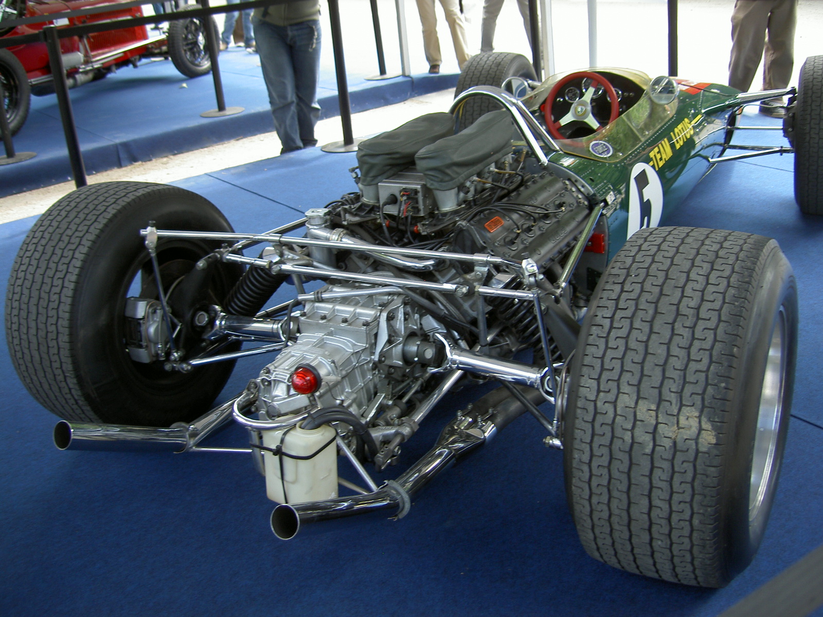
Figure: The Lotus 49, view from the rear. The Lotus 49 was one of the last Formula One cars before the introduction of aerodynamic aids.

So when it comes to our ability to compute we are extraordinary, not compute in our conscious mind, but the underlying neuron firings that underpin both our consciousness, our subconsciousness as well as our motor control etc.

If we think of ourselves as vehicles, then we are massively overpowered. Our ability to generate derived information from raw fuel is extraordinary. Intellectually we have formula one engines.

But in terms of our ability to deploy that computation in actual use, to share the results of what we have inferred, we are very limited. So when you imagine the F1 car that represents a psyche, think of an F1 car with bicycle wheels.

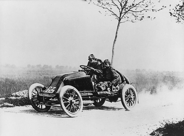
Figure: Marcel Renault races a Renault 40 cv during the Paris-Madrid race, an early Grand Prix, in 1903. Marcel died later in the race after missing a warning flag for a sharp corner at Couhé Vérac, likely due to dust reducing visibility.

Just think of the control a driver would have to have to deploy such power through such a narrow channel of traction. That is the beauty and the skill of the human mind.

In contrast, our computers are more like go-karts. Underpowered, but with well-matched tires. They can communicate far more fluidly. They are more efficient, but somehow less extraordinary, less beautiful.

Figure: Caleb McDuff driving for WIX Silence Racing.

Human Communication

For human conversation to work, we require an internal model of who we are speaking to. We model each other, and combine our sense of who they are, who they think we are, and what has been said. This is our approach to dealing with the limited bandwidth connection we have. Empathy and understanding of intent. Mental dispositional concepts are used to augment our limited communication bandwidth.

Fritz Heider referred to the important point of a conversation as being that they are happenings that are “psychologically represented in each of the participants” (his emphasis) (Heider, 1958).

Bandwidth Constrained Conversations

Figure: Conversation relies on internal models of other individuals.

Figure: Misunderstanding of context and who we are talking to leads to arguments.

Embodiment factors imply that, in our communication between humans, what is not said is, perhaps, more important than what is said. To communicate with each other we need to have a model of who each of us are.

To aid this, in society, we are required to perform roles. Whether as a parent, a teacher, an employee or a boss. Each of these roles requires that we conform to certain standards of behaviour to facilitate communication between ourselves.

Control of self is vitally important to these communications.

The high availability of data available to humans undermines human-to-human communication channels by providing new routes to undermining our control of self.

Figure: The Global storage capacity between 1986 and 2007 Hilbert and López (2011)

A Six Word Novel

For sale: baby shoes, never worn

Figure: Consider the six word novel, apocraphally credited to Ernest Hemingway, “For sale: baby shoes, never worn.” To understand what that means to a human, you need a great deal of additional context. Context that is not directly accessible to a machine that has not got both the evolved and contextual understanding of our own condition to realize both the implication of the advert and what that implication means emotionally to the previous owner.

But this is a very different kind of intelligence than ours. A computer cannot understand the depth of the Ernest Hemingway’s apocryphal six word novel: “For Sale, Baby Shoes, Never worn,” because it isn’t equipped with that ability to model the complexity of humanity that underlies that statement.

Computer Conversations

Figure: Conversation relies on internal models of other individuals.

Figure: Misunderstanding of context and who we are talking to leads to arguments.

Similarly, we find it difficult to comprehend how computers are making decisions. Because they do so with more data than we can possibly imagine.

In many respects, this is not a problem, it’s a good thing. Computers and us are good at different things. But when we interact with a computer, when it acts in a different way to us, we need to remember why.

Just as the first step to getting along with other humans is understanding other humans, so it needs to be with getting along with our computers.

Embodiment factors explain why, at the same time, computers are so impressive in simulating our weather, but so poor at predicting our moods. Our complexity is greater than that of our weather, and each of us is tuned to read and respond to one another.

Their intelligence is different. It is based on very large quantities of data that we cannot absorb. Our computers don’t have a complex internal model of who we are. They don’t understand the human condition. They are not tuned to respond to us as we are to each other.

Embodiment factors encapsulate a profound thing about the nature of humans. Our locked in intelligence means that we are striving to communicate, so we put a lot of thought into what we’re communicating with. And if we’re communicating with something complex, we naturally anthropomorphize them.

We give our dogs, our cats and our cars human motivations. We do the same with our computers. We anthropomorphize them. We assume that they have the same objectives as us and the same constraints. They don’t.

This means, that when we worry about artificial intelligence, we worry about the wrong things. We fear computers that behave like more powerful versions of ourselves that will struggle to outcompete us.

In reality, the challenge is that our computers cannot be human enough. They cannot understand us with the depth we understand one another. They drop below our cognitive radar and operate outside our mental models.

The real danger is that computers don’t anthropomorphize. They’ll make decisions in isolation from us without our supervision, because they can’t communicate truly and deeply with us.

Evolved Relationship with Information

The high bandwidth of computers has resulted in a close relationship between the computer and data. Large amounts of information can flow between the two. The degree to which the computer is mediating our relationship with data means that we should consider it an intermediary.

Originaly our low bandwith relationship with data was affected by two characteristics. Firstly, our tendency to over-interpret driven by our need to extract as much knowledge from our low bandwidth information channel as possible. Secondly, by our improved understanding of the domain of mathematical statistics and how our cognitive biases can mislead us.

With this new set up there is a potential for assimilating far more information via the computer, but the computer can present this to us in various ways. If it’s motives are not aligned with ours then it can misrepresent the information. This needn’t be nefarious it can be simply as a result of the computer pursuing a different objective from us. For example, if the computer is aiming to maximize our interaction time that may be a different objective from ours which may be to summarize information in a representative manner in the shortest possible length of time.

For example, for me, it was a common experience to pick up my telephone with the intention of checking when my next appointment was, but to soon find myself distracted by another application on the phone, and end up reading something on the internet. By the time I’d finished reading, I would often have forgotten the reason I picked up my phone in the first place.

There are great benefits to be had from the huge amount of information we can unlock from this evolved relationship between us and data. In biology, large scale data sharing has been driven by a revolution in genomic, transcriptomic and epigenomic measurement. The improved inferences that can be drawn through summarizing data by computer have fundamentally changed the nature of biological science, now this phenomenon is also infuencing us in our daily lives as data measured by happenstance is increasingly used to characterize us.

Better mediation of this flow actually requires a better understanding of human-computer interaction. This in turn involves understanding our own intelligence better, what its cognitive biases are and how these might mislead us.

For further thoughts see Guardian article on marketing in the internet era from 2015.

You can also check my blog post on System Zero. also from 2015.

New Flow of Information

Classically the field of statistics focussed on mediating the relationship between the machine and the human. Our limited bandwidth of communication means we tend to over-interpret the limited information that we are given, in the extreme we assign motives and desires to inanimate objects (a process known as anthropomorphizing). Much of mathematical statistics was developed to help temper this tendency and understand when we are valid in drawing conclusions from data.

Figure: The trinity of human, data and computer, and highlights the modern phenomenon. The communication channel between computer and data now has an extremely high bandwidth. The channel between human and computer and the channel between data and human is narrow. New direction of information flow, information is reaching us mediated by the computer. The focus on classical statistics reflected the importance of the direct communication between human and data. The modern challenges of data science emerge when that relationship is being mediated by the machine.

Data science brings new challenges. In particular, there is a very large bandwidth connection between the machine and data. This means that our relationship with data is now commonly being mediated by the machine. Whether this is in the acquisition of new data, which now happens by happenstance rather than with purpose, or the interpretation of that data where we are increasingly relying on machines to summarise what the data contains. This is leading to the emerging field of data science, which must not only deal with the same challenges that mathematical statistics faced in tempering our tendency to over interpret data, but must also deal with the possibility that the machine has either inadvertently or malisciously misrepresented the underlying data.

The Centrifugal Governor

Figure: Centrifugal governor as held by “Science” on Holborn Viaduct

Boulton and Watt’s Steam Engine

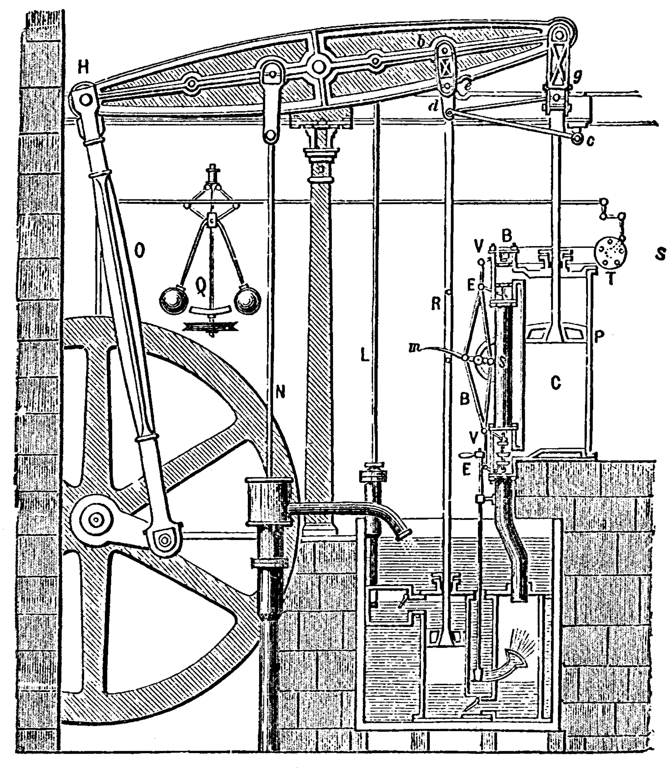
Figure: Watt’s Steam Engine which made Steam Power Efficient and Practical.

James Watt’s steam engine contained an early machine learning device. In the same way that modern systems are component based, his engine was composed of components. One of which is a speed regulator sometimes known as Watt’s governor. The two balls in the center of the image, when spun fast, rise, and through a linkage mechanism.

The centrifugal governor was made famous by Boulton and Watt when it was deployed in the steam engine. Studying stability in the governor is the main subject of James Clerk Maxwell’s paper on the theoretical analysis of governors (Maxwell, 1867). This paper is a founding paper of control theory. In an acknowledgment of its influence, Wiener used the name cybernetics to describe the field of control and communication in animals and the machine (Wiener, 1948). Cybernetics is the Greek word for governor, which comes from the latin for helmsman.

A governor is one of the simplest artificial intelligence systems. It senses the speed of an engine, and acts to change the position of the valve on the engine to slow it down.

Although it’s a mechanical system a governor can be seen as automating a role that a human would have traditionally played. It is an early example of artificial intelligence.

The centrifugal governor has several parameters, the weight of the balls used, the length of the linkages and the limits on the balls movement.

Two principle differences exist between the centrifugal governor and artificial intelligence systems of today.

1. The centrifugal governor is a physical system and it is an integral part of a wider physical system that it regulates (the engine).
2. The parameters of the governor were set by hand, our modern artificial intelligence systems have their parameters set by data.

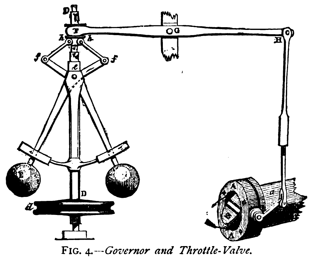
Figure: The centrifugal governor, an early example of a decision making system. The parameters of the governor include the lengths of the linkages (which effect how far the throttle opens in response to movement in the balls), the weight of the balls (which effects inertia) and the limits of to which the balls can rise.

This has the basic components of sense and act that we expect in an intelligent system, and this system saved the need for a human operator to manually adjust the system in the case of overspeed. Overspeed has the potential to destroy an engine, so the governor operates as a safety device.

The first wave of automation did bring about sabotoage as a worker’s response. But if machinery was sabotaged, for example, if the linkage between sensor (the spinning balls) and action (the valve closure) was broken, this would be obvious to the engine operator at start up time. The machine could be repaired before operation.

What is Machine Learning?

Machine learning allows us to extract knowledge from data to form a prediction.

\[\text{data} + \text{model} \stackrel{\text{compute}}{\rightarrow} \text{prediction}\]

A machine learning prediction is made by combining a model with data to form the prediction. The manner in which this is done gives us the machine learning algorithm.

Machine learning models are mathematical models which make weak assumptions about data, e.g. smoothness assumptions. By combining these assumptions with the data, we observe we can interpolate between data points or, occasionally, extrapolate into the future.

Machine learning is a technology which strongly overlaps with the methodology of statistics. From a historical/philosophical view point, machine learning differs from statistics in that the focus in the machine learning community has been primarily on accuracy of prediction, whereas the focus in statistics is typically on the interpretability of a model and/or validating a hypothesis through data collection.

The rapid increase in the availability of compute and data has led to the increased prominence of machine learning. This prominence is surfacing in two different but overlapping domains: data science and artificial intelligence.

From Model to Decision

The real challenge, however, is end-to-end decision making. Taking information from the environment and using it to drive decision making to achieve goals.

The Big Data Paradox

The big data paradox is the modern phenomenon of “as we collect more data, we understand less.” It is emerging in several domains, political polling, characterization of patients for trials data, monitoring twitter for political sentiment.

I like to think of the phenomenon as relating to the notion of “can’t see the wood for the trees.” Classical statistics, with randomized controlled trials, improved society’s understanding of data. It improved our ability to monitor the forest, to consider population health, voting patterns etc. It is critically dependent on active approaches to data collection that deal with confounders. This data collection can be very expensive.

In business today, it is still the gold standard, A/B tests are used to understand the effect of an intervention on revenue or customer capture or supply chain costs.

Figure: New beech leaves growing in the Gribskov Forest in the northern part of Sealand, Denmark. Photo from wikimedia commons by Malene Thyssen, http://commons.wikimedia.org/wiki/User:Malene.

The new phenomenon is happenstance data. Data that is not actively collected with a question in mind. As a result, it can mislead us. For example, if we assume the politics of active users of twitter is reflective of the wider population’s politics, then we may be misled.

However, this happenstance data often allows us to characterise a particular individual to a high degree of accuracy. Classical statistics was all about the forest, but big data can often become about the individual tree. As a result we are misled about the situation.

The phenomenon is more dangerous, because our perception is that we are characterizing the wider scenario with ever increasing accuracy. Whereas we are just becoming distracted by detail that may or may not be pertinent to the wider situation.

This is related to our limited bandwidth as humans, and the ease with which we are distracted by detail. The data-inattention-cognitive-bias.

Complexity in Action

As an exercise in understanding complexity, watch the following video. You will see the basketball being bounced around, and the players moving. Your job is to count the passes of those dressed in white and ignore those of the individuals dressed in black.

Figure: Daniel Simon’s famous illusion “monkey business.” Focus on the movement of the ball distracts the viewer from seeing other aspects of the image.

In a classic study Simons and Chabris (1999) ask subjects to count the number of passes of the basketball between players on the team wearing white shirts. Fifty percent of the time, these subjects don’t notice the gorilla moving across the scene.

The phenomenon of inattentional blindness is well known, e.g in their paper Simons and Charbris quote the Hungarian neurologist, Rezsö Bálint,

It is a well-known phenomenon that we do not notice anything happening in our surroundings while being absorbed in the inspection of something; focusing our attention on a certain object may happen to such an extent that we cannot perceive other objects placed in the peripheral parts of our visual field, although the light rays they emit arrive completely at the visual sphere of the cerebral cortex.

Rezsö Bálint 1907 (translated in Husain and Stein 1988, page 91)

When we combine the complexity of the world with our relatively low bandwidth for information, problems can arise. Our focus on what we perceive to be the most important problem can cause us to miss other (potentially vital) contextual information.

This phenomenon is known as selective attention or ‘inattentional blindness.’

Figure: For a longer talk on inattentional bias from Daniel Simons see this video.

Data Selective Attention Bias

We are going to see how inattention biases can play out in data analysis by going through a simple example. The analysis involves body mass index and activity information.

BMI Steps Data

The BMI Steps example is taken from Yanai and Lercher (2020). We are given a data set of body-mass index measurements against step counts. For convenience we have packaged the data so that it can be easily downloaded.

import pods

data = pods.datasets.bmi_steps()
X = data['X'] 
y = data['Y']

It is good practice to give our variables interpretable names so that the analysis may be clearly understood by others. Here the steps count is the first dimension of the covariate, the bmi is the second dimension and the gender is stored in y with 1 for female and 0 for male.

steps = X[:, 0]
bmi = X[:, 1]
gender = y[:, 0]

We can check the mean steps and the mean of the BMI.

print('Steps mean is {mean}.'.format(mean=steps.mean()))

print('BMI mean is {mean}.'.format(mean=bmi.mean()))

BMI Steps Data Analysis

We can also separate out the means from the male and female populations. In python this can be done by setting male and female indices as follows.

male_ind = (gender==0)
female_ind = (gender==1)

And now we can extract the variables for the two populations.

male_steps = steps[male_ind]
male_bmi = bmi[male_ind]

And as before we compute the mean.

print('Male steps mean is {mean}.'.format(mean=male_steps.mean()))

print('Male BMI mean is {mean}.'.format(mean=male_bmi.mean()))

Similarly, we can get the same result for the female portion of the populaton.

female_steps = steps[female_ind]
female_bmi = bmi[female_ind]

print('Female steps mean is {mean}.'.format(mean=female_steps.mean()))

print('Female BMI mean is {mean}.'.format(mean=female_bmi.mean()))

Interesting, the female BMI average is slightly higher than the male BMI average. The number of steps in the male group is higher than that in the female group. Perhaps the steps and the BMI are anti-correlated. The more steps, the lower the BMI.

Python provides a statistics package. We’ll import this in python so that we can try and understand the correlation between the steps and the BMI.

from scipy.stats import pearsonr

corr, _ = pearsonr(steps, bmi)
print("Pearson's overall correlation: {corr}".format(corr=corr))

male_corr, _ = pearsonr(male_steps, male_bmi)
print("Pearson's correlation for males: {corr}".format(corr=male_corr))

female_corr, _ = pearsonr(female_steps, female_bmi)
print("Pearson's correlation for females: {corr}".format(corr=female_corr))

A Hypothesis as a Liability

This analysis is from an article titled “A Hypothesis as a Liability” (Yanai and Lercher, 2020), they start their article with the following quite from Herman Hesse.

“ ‘When someone seeks,’ said Siddhartha, ‘then it easily happens that his eyes see only the thing that he seeks, and he is able to find nothing, to take in nothing. […] Seeking means: having a goal. But finding means: being free, being open, having no goal.’ ”

Hermann Hesse

Their idea is that having a hypothesis can constrain our thinking. However, in answer to their paper Felin et al. (2021) argue that some form of hypothesis is always necessary, suggesting that a hypothesis can be a liability

My view is captured in the introductory chapter to an edited volume on computational systems biology that I worked on with Mark Girolami, Magnus Rattray and Guido Sanguinetti.

Figure: Quote from Lawrence (2010) highlighting the importance of interaction between data and hypothesis.

Popper nicely captures the interaction between hypothesis and data by relating it to the chicken and the egg. The important thing is that these two co-evolve.

Number Theatre

Unfortunately, we don’t always have time to wait for this process to converge to an answer we can all rely on before a decision is required.

Not only can we be misled by data before a decision is made, but sometimes we can be misled by data to justify the making of a decision. David Spiegelhalter refers to the phenomenon of “Number Theatre” in a conversation with Andrew Marr from May 2020 on the presentation of data.

Figure: Professor Sir David Spiegelhalter on Andrew Marr on 10th May 2020 speaking about some of the challengers around data, data presentation, and decision making in a pandemic. David mentions number theatre at 9 minutes 10 seconds.

Data Theatre

Data Theatre exploits data inattention bias to present a particular view on events that may misrepresents through selective presentation. Statisticians are one of the few groups that are trained with a sufficient degree of data skepticism. But it can also be combatted through ensuring there are domain experts present, and that they can speak freely.

Figure: The pheonomenon of number theatre or data theatre was described by David Spiegelhalter and is nicely sumamrized by Martin Robbins in this sub-stack article https://martinrobbins.substack.com/p/data-theatre-why-the-digital-dashboards.

The best book I have found for teaching the skeptical sense of data that underlies the statisticians craft is David Spiegelhalter’s Art of Statistics.

The Art of Statistics

Figure: The Art of Statistics by David Spiegelhalter is an excellent read on the pitfalls of data interpretation.

David’s (Spiegelhalter, 2019) book brings important examples from statistics to life in an intelligent and entertaining way. It is highly readable and gives an opportunity to fast-track towards the important skill of data-skepticism that is the mark of a professional statistician.