Preserving Human Voices and Faces
Abstract
The information revolution — and AI is its latest phase — is like a nutrient flood in an ecosystem. Algae are the organisms best placed to exploit nitrogen, and when nitrogen floods in they bloom rapidly, consuming the oxygen and crowding out diversity. In 1971 Herbert Simon warned that a wealth of information creates a poverty of attention. Today that poverty is acute. But the very quality that makes us bandwidth-limited also makes us irreplaceable: we carry the knowledge that comes from being mortal and vulnerable. This talk explores the embodiment factor — the million-to-one gap between how fast we communicate and how fast machines do — and argues that human culture, like ecology, carries complexity that cannot be scaled or uploaded. The challenge before us is to ensure the information bloom does not destroy the diverse ecosystem of human voice and face.
Information Overload and the Algal Bloom
There is a phenomenon ecologists call an algal bloom. Algae are the organisms in our waterways best positioned to exploit nitrogen. When nitrogen floods into an ecosystem — from agricultural runoff, from fertiliser-laden rainfall — algae do what they are optimised to do: they grow. Rapidly, voraciously, they spread across the surface of the water. To the casual observer it can look impressive, even beautiful. But the bloom is catastrophic. It consumes the dissolved oxygen. It kills the fish. It crowds out every other form of life. The very success of the algae — their perfect adaptation to exploit a suddenly abundant resource — destroys the ecosystem that once sustained that diversity.
I want to suggest that we are witnessing something very similar in the domain of information. The information revolution — and AI is simply its latest and most powerful phase — does not straightforwardly enrich us. Like nitrogen flooding a waterway, it can overwhelm the ecosystem of human attention, human culture, and human voice.
The economist and computer scientist Herbert Simon saw this coming fifty years ago. In 1971 he wrote:
A wealth of information creates a poverty of attention. Information is like nitrogen — when it floods in, the organisms best equipped to exploit it grow fastest, and what is lost is the diversity of the ecosystem. The question this conference asks — how do we preserve human voices and faces? — is precisely the right question to be asking at this moment. Because human attention, and the culture it sustains, is what the bloom threatens to destroy.
See Lawrence (2024) Simon, Herbert p. 140.
The Attention Economy
Human intelligence is locked-in. It’s bandwidth restricted. This makes it a bottleneck in the attention economy.
Herbert Simon on Information
What information consumes is rather obvious: it consumes the attention of its recipients. Hence a wealth of information creates a poverty of attention …
Simon (1971)
The attention economy was a phenomenon described in 1971 by the American computer scientist Herbert Simon. He saw the coming information revolution and wrote that a wealth of information would create a poverty of attention. Too much information means that human attention becomes the scarce resource, the bottleneck. It becomes the gold in the attention economy.
The power associated with control of information dates back to the invention of writing. By pressing reeds into clay tablets Sumerian scribes stored information and controlled the flow of information.
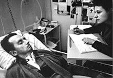

Figure: Jean Dominique Bauby was the Editor in Chief of the French Elle Magazine, he suffered a stroke that destroyed his brainstem, leaving him only capable of moving one eye. Jean Dominique became a victim of locked in syndrome.
Incredibly, Jean Dominique wrote his book after he became locked in. It took him 10 months of four hours a day to write the book. Each word took two minutes to write.
The idea behind embodiment factors is that we are all in that situation. While not as extreme as for Bauby, we all have somewhat of a locked in intelligence.
See Lawrence (2024) Bauby, Jean Dominique p. 9–11, 18, 90, 99-101, 133, 186, 212–218, 234, 240, 251–257, 318, 368–369.
Bauby and Shannon
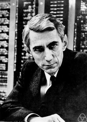
Figure: Claude Shannon developed information theory which allows us to quantify how much Bauby can communicate. This allows us to compare how locked in he is to us.
See Lawrence (2024) Shannon, Claude p. 10, 30, 61, 74, 98, 126, 134, 140, 143, 149, 260, 264, 269, 277, 315, 358, 363.
Embodiment Factors
| bits/min | billions | 2,000 |
|
billion calculations/s |
~100 | a billion |
| embodiment | 20 minutes | 5 billion years |
Figure: Embodiment factors are the ratio between our ability to compute and our ability to communicate. Relative to the machine we are also locked in. In the table we represent embodiment as the length of time it would take to communicate one second’s worth of computation. For computers it is a matter of minutes, but for a human, it is a matter of thousands of millions of years. See also “Living Together: Mind and Machine Intelligence” Lawrence (2017)
There is a fundamental limit placed on our intelligence based on our ability to communicate. Claude Shannon founded the field of information theory. The clever part of this theory is it allows us to separate our measurement of information from what the information pertains to.1
Shannon measured information in bits. One bit of information is the amount of information I pass to you when I give you the result of a coin toss. Shannon was also interested in the amount of information in the English language. He estimated that on average a word in the English language contains 12 bits of information.
Given typical speaking rates, that gives us an estimate of our ability to communicate of around 100 bits per second (Reed and Durlach, 1998). Computers on the other hand can communicate much more rapidly. Current wired network speeds are around a billion bits per second, ten million times faster.
When it comes to compute though, our best estimates indicate our computers are slower. A typical modern computer can process make around 100 billion floating-point operations per second, each floating-point operation involves a 64 bit number. So the computer is processing around 6,400 billion bits per second.
It’s difficult to get similar estimates for humans, but by some estimates the amount of compute we would require to simulate a human brain is equivalent to that in the UK’s fastest computer (Ananthanarayanan et al., 2009), the MET office machine in Exeter, which in 2018 ranked as the 11th fastest computer in the world. That machine simulates the world’s weather each morning, and then simulates the world’s climate in the afternoon. It is a 16-petaflop machine, processing around 1,000 trillion bits per second.
See Lawrence (2024) embodiment factor p. 13, 29, 35, 79, 87, 105, 197, 216-217, 249, 269, 353, 369.
A Six Word Novel

Figure: Consider the six-word novel, apocryphally credited to Ernest Hemingway, “For sale: baby shoes, never worn.” To understand what that means to a human, you need a great deal of additional context. Context that is not directly accessible to a machine that has not got both the evolved and contextual understanding of our own condition to realize both the implication of the advert and what that implication means emotionally to the previous owner.
See Lawrence (2024) baby shoes p. 368.
But this is a very different kind of intelligence than ours. A computer cannot understand the depth of the Ernest Hemingway’s apocryphal six-word novel: “For Sale, Baby Shoes, Never worn,” because it isn’t equipped with that ability to model the complexity of humanity that underlies that statement.
New Flow of Information
Classically the field of statistics focused on mediating the relationship between the machine and the human. Our limited bandwidth of communication means we tend to over-interpret the limited information that we are given, in the extreme we assign motives and desires to inanimate objects (a process known as anthropomorphizing). Much of mathematical statistics was developed to help temper this tendency and understand when we are valid in drawing conclusions from data.
Figure: The trinity of human, data, and computer, and highlights the modern phenomenon. The communication channel between computer and data now has an extremely high bandwidth. The channel between human and computer and the channel between data and human is narrow. New direction of information flow, information is reaching us mediated by the computer. The focus on classical statistics reflected the importance of the direct communication between human and data. The modern challenges of data science emerge when that relationship is being mediated by the machine.
Data science brings new challenges. In particular, there is a very large bandwidth connection between the machine and data. This means that our relationship with data is now commonly being mediated by the machine. Whether this is in the acquisition of new data, which now happens by happenstance rather than with purpose, or the interpretation of that data where we are increasingly relying on machines to summarize what the data contains. This is leading to the emerging field of data science, which must not only deal with the same challenges that mathematical statistics faced in tempering our tendency to over interpret data but must also deal with the possibility that the machine has either inadvertently or maliciously misrepresented the underlying data.
See Lawrence (2024) topography, information p. 34-9, 43-8, 57, 62, 104, 115-16, 127, 140, 192, 196, 199, 291, 334, 354-5. See Lawrence (2024) anthropomorphization (‘anthrox’) p. 30-31, 90-91, 93-4, 100, 132, 148, 153, 163, 216-17, 239, 276, 326, 342.
Human Analogue Machine
Recent breakthroughs in generative models, particularly large language models, have enabled machines that, for the first time, can converse plausibly with other humans.
The Apollo guidance computer provided Armstrong with an analogy when he landed it on the Moon. He controlled it through a stick which provided him with an analogy. The analogy is based in the experience that Amelia Earhart had when she flew her plane. Armstrong’s control exploited his experience as a test pilot flying planes that had control columns which were directly connected to their control surfaces.
Figure: The human analogue machine is the new interface that large language models have enabled the human to present. It has the capabilities of the computer in terms of communication, but it appears to present a “human face” to the user in terms of its ability to communicate on our terms. (Image quite obviously not drawn by generative AI!)
The generative systems we have produced do not provide us with the “AI” of science fiction. Because their intelligence is based on emulating human knowledge. Through being forced to reproduce our literature and our art they have developed aspects which are analogous to the cultural proxy truths we use to describe our world.
These machines are to humans what the MONIAC was the British economy. Not a replacement, but an analogue computer that captures some aspects of humanity while providing advantages of high bandwidth of the machine.
See Lawrence (2024) ignorance: HAMs p. 347. See Lawrence (2024) test pilot p. 163-8, 189, 190, 192-3, 196, 197, 200, 211, 245.
Bandwidth vs Complexity
The computer communicates in Gigabits per second, One way of imagining just how much slower we are than the machine is to look for something that communicates in nanobits per second.
|
|||
| bits/min | \(100 \times 10^{-9}\) | \(2,000\) | \(600 \times 10^9\) |
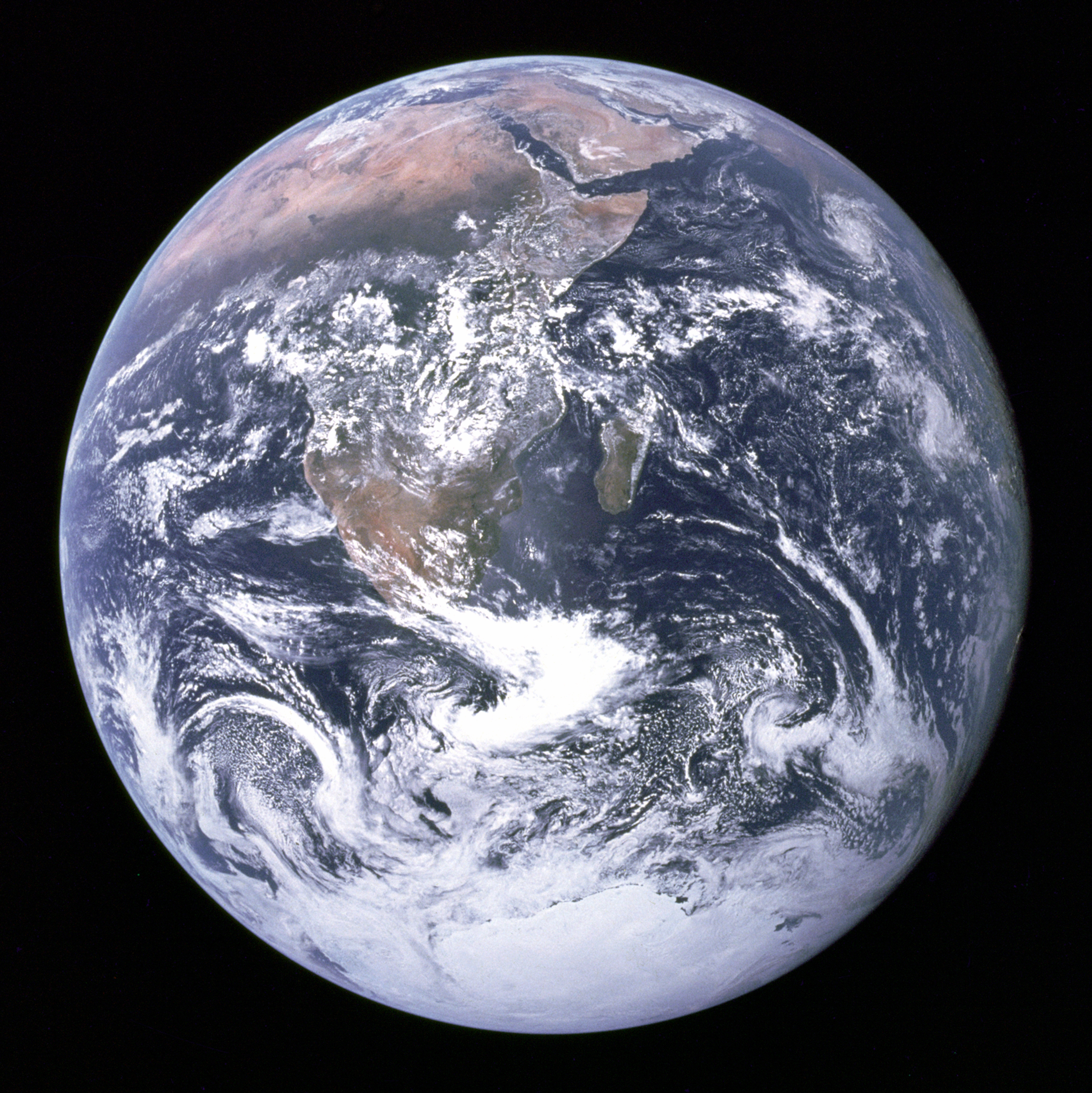
Figure: When we look at communication rates based on the information passing from one human to another across generations through their genetics, we see that computers watching us communicate is roughly equivalent to us watching organisms evolve. Estimates of germline mutation rates taken from Scally (2016).
Figure: Bandwidth vs Complexity.
The challenge we face is that while speed is on the side of the machine, complexity is on the side of our ecology. Many of the risks we face are associated with the way our speed undermines our ecology and the machines speed undermines our human culture.
See Lawrence (2024) Human evolution rates p. 98-99. See Lawrence (2024) Psychological representation of Ecologies p. 323-327.
The Atomic Human
Figure: The Atomic Eye, by slicing away aspects of the human that we used to believe to be unique to us, but are now the preserve of the machine, we learn something about what it means to be human.
The development of what some are calling intelligence in machines, raises questions around what machine intelligence means for our intelligence. The idea of the atomic human is derived from Democritus’s atomism.
In the fifth century bce the Greek philosopher Democritus posed a question about our physical universe. He imagined cutting physical matter into pieces in a repeated process: cutting a piece, then taking one of the cut pieces and cutting it again so that each time it becomes smaller and smaller. Democritus believed this process had to stop somewhere, that we would be left with an indivisible piece. The Greek word for indivisible is atom, and so this theory was called atomism.
The Atomic Human considers the same question, but in a different domain, asking: As the machine slices away portions of human capabilities, are we left with a kernel of humanity, an indivisible piece that can no longer be divided into parts? Or does the human disappear altogether? If we are left with something, then that uncuttable piece, a form of atomic human, would tell us something about our human spirit.
See Lawrence (2024) atomic human, the p. 13.
Conclusion
Human culture is an ecology. It has evolved over tens of thousands of years and carries complexity that we cannot fully articulate, because that complexity lives in relationships, communities, traditions, liturgies, and stories told across generations — in all the things that cannot be uploaded or scaled.
The question before us is whether we can bring custodial wisdom to this new moment. Can we ensure that what floods in — the nitrogen of our digital age — feeds genuine growth rather than a catastrophic bloom?
The answer is yes, but only if we are clear about what we are protecting and why. We are protecting the space for the atomic human — for that indivisible kernel of human experience that no machine can replicate, because no machine has lived. Our voices and faces are worth preserving precisely because they carry what cannot be transferred: the knowledge that comes from being mortal, from being vulnerable, from being one of us.
Thanks!
For more information on these subjects and more you might want to check the following resources.
- company: Trent AI
- book: The Atomic Human
- twitter: @lawrennd
- podcast: The Talking Machines
- newspaper: Guardian Profile Page
- blog: http://inverseprobability.com
References
the challenge of understanding what information pertains to is known as knowledge representation.↩︎