The Inaccessible Game
Abstract
Most games rely on an external adjudicator. That is, an observer outside the system who defines outcomes, measures states, and applies rules. What happens when we forbid this?
This talk develops the “inaccessible game,” an information-theoretic dynamical system that forbids external adjudication. We introduce the game and present the no-barber principle which supports us when selecting the game’s rules.
We explain how structure emerges from these foundations and speculate on why this framing might be useful in understanding the limits of information infrastructures and the limits of intelligence.
Artificial General Vehicle
Artificial General Vehicle
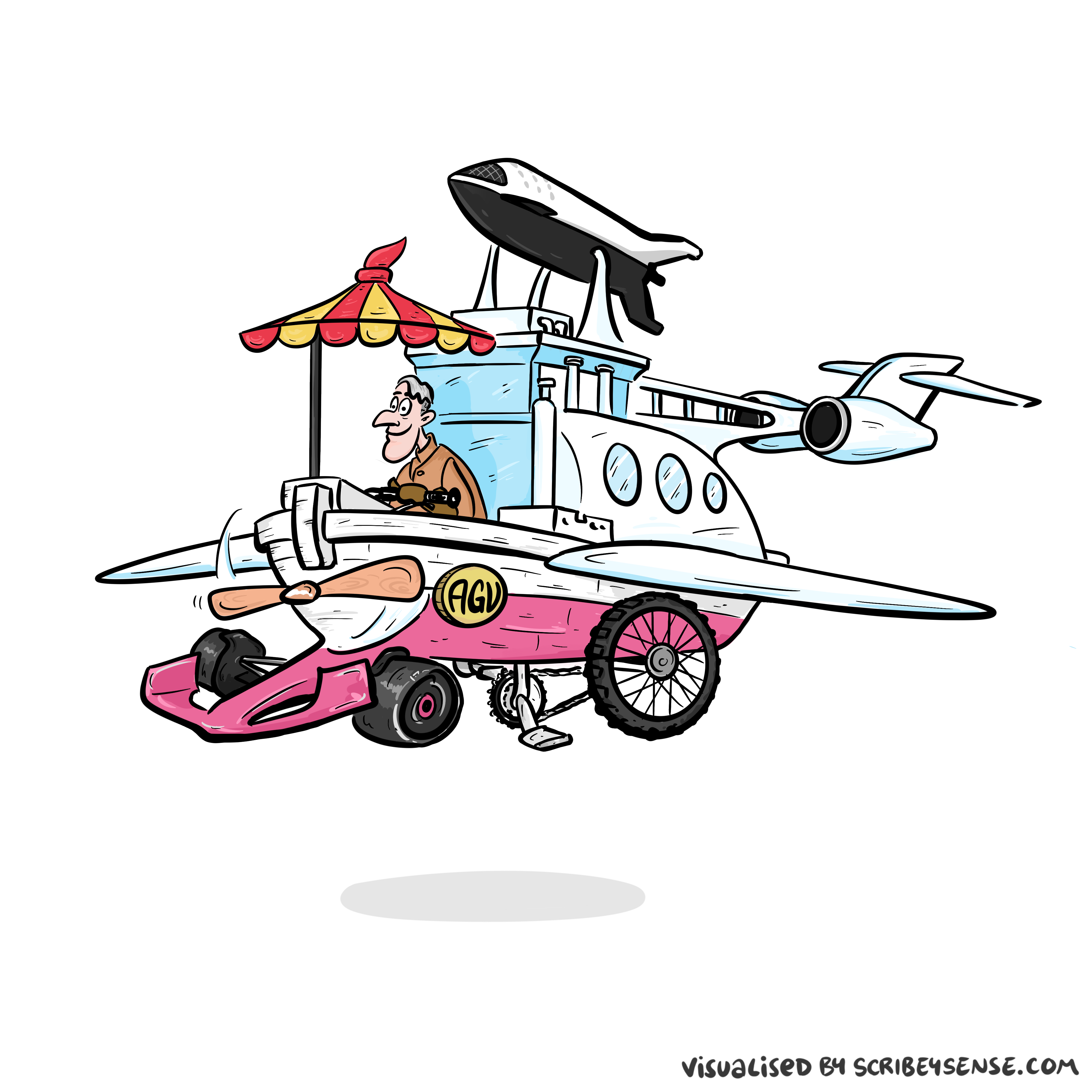

Figure: The notion of artificial general intelligence is as absurd as the notion of an artificial general vehicle - no single vehicle is optimal for every journey. (Illustration by Dan Andrews inspired by a conversation about “The Atomic Human” Lawrence (2024))
This illustration was created by Dan Andrews inspired by a conversation about “The Atomic Human” book. The drawing emerged from discussions with Dan about the flawed concept of artificial general intelligence and how it parallels the absurd idea of a single vehicle optimal for all journeys. The vehicle itself is inspired by shared memories of Professor Pat Pending in Hanna Barbera’s Wacky Races.
I often turn up to talks with my Brompton bicycle. Embarrassingly I even took it to Google which is only a 30 second walk from King’s Cross station. That made me realise it’s become a sort of security blanket. I like having it because it’s such a flexible means of transport.
But is the Brompton an “artificial general vehicle?” A vehicle that can do everything? Unfortunately not, for example it’s not very good for flying to the USA. There is no artificial general vehicle that is optimal for every journey. Similarly there is no such thing as artificial general intelligence. The idea is artificial general nonsense.
That doesn’t mean there aren’t different principles to intelligence we can look at. Just like vehicles have principles that apply to them. When designing vehicles we need to think about air resistance, friction, power. We have developed solutions such as wheels, different types of engines and wings that are deployed across different vehicles to achieve different results.
Intelligence is similar. The notion of artificial general intelligence is fundamentally eugenic. It builds on Spearman’s term “general intelligence” which is part of a body of literature that was looking to assess intelligence in the way we assess height. The objective then being to breed greater intelligences (Lyons, 2022).
The Atomic Human
Figure: The Atomic Eye, by slicing away aspects of the human that we used to believe to be unique to us, but are now the preserve of the machine, we learn something about what it means to be human.
The development of what some are calling intelligence in machines, raises questions around what machine intelligence means for our intelligence. The idea of the atomic human is derived from Democritus’s atomism.
In the fifth century bce the Greek philosopher Democritus posed a question about our physical universe. He imagined cutting physical matter into pieces in a repeated process: cutting a piece, then taking one of the cut pieces and cutting it again so that each time it becomes smaller and smaller. Democritus believed this process had to stop somewhere, that we would be left with an indivisible piece. The Greek word for indivisible is atom, and so this theory was called atomism.
The Atomic Human considers the same question, but in a different domain, asking: As the machine slices away portions of human capabilities, are we left with a kernel of humanity, an indivisible piece that can no longer be divided into parts? Or does the human disappear altogether? If we are left with something, then that uncuttable piece, a form of atomic human, would tell us something about our human spirit.
See Lawrence (2024) atomic human, the p. 13.
Embodiment Factors: Walking vs Light Speed
Imagine human communication as moving at walking pace. The average person speaks about 160 words per minute, which is roughly 2000 bits per minute. If we compare this to walking speed, roughly 1 m/s we can think of this as the speed at which our thoughts can be shared with others.
Compare this to machines. When computers communicate, their bandwidth is 600 billion bits per minute. Three hundred million times faster than humans or the equiavalent of \(3 \times 10 ^{8}\). In twenty minutes we could be a kilometer down the road, where as the computer can go to the Sun and back again..
This difference is not just only about speed of communication, but about embodiment. Our intelligence is locked in by our biology: our brains may process information rapidly, but our ability to share those thoughts is limited to the slow pace of speech or writing. Machines, in comparison, seem able to communicate their computations almost instantaneously, anywhere.
So, the embodiment factor is the ratio between the time it takes to think a thought and the time it takes to communicate it. For us, it’s like walking; for machines, it’s like moving at light speed. This difference means that most direct comparisons between human and machine need to be carefully made. Because for humans not the size of our communication bandwidth that counts, but it’s how we overcome that limitation..
Formalising Information Topography
In The Atomic Human (Lawrence, 2024), the concept of an information topography was introduced as a metaphor: “In geography, the topography is the configuration of natural and man-made features in the landscape… These questions are framed by the topography. An information topography is similar, but instead of the movement of goods, water and people, it dictates the movement of information.”
However, no formal mathematical definition was given. The inaccessible game is an attempt to provide one.
The Munchkin Provision
Without such consistency, we would require what we might call a “Munchkin provision.” In the Munchkin card game (Jackson, 2001), it is acknowledged that the cards and rules may be inconsistent. Their resolution?
Any other disputes should be settled by loud arguments, with the owner of the game having the last word.
Munckin Rules (Jackson, 2001)
While this works for card games, it’s unsatisfying for foundational mathematics. We want our game to be internally consistent, not requiring an external referee to resolve paradoxes.
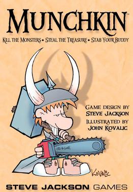
Figure: The Munchkin card came has both cards and rules. The game explicitly acknowledges that this can lead to inconsistencies which should be resolved by the game owner.
A Tautology
Self-governing systems cannot refer to external arbitration.
While this is a tautology, we will try to formalise it through information theory. The key question is: what mathematical structure is forced on a system that cannot appeal to external adjudication?
The No-Barber Principle
In 1901 Bertrand Russell introduced a paradox: if a barber shaves everyone in the village who does not shave themselves, does the barber shave themselves? The paradox arises when a definition quantifies over a totality that includes the defining rule itself.
We propose a similar constraint for the inaccessible game: the foundational rules must not refer to anything outside themselves for adjudication or reference. Or in other words there can be no external structure. We call this the “no-barber principle” (Lawrence, 2026a).
The no-barber principle says that admissible rules must be internally adjudicable: they depend only on quantities definable from within the system’s internal language, without requiring e.g. an external observer to define the co-ordinates or a privileged decomposition.
Baez-Fritz-Leinster Characterization of Information Loss
Before introducing our fourth axiom, we need to understand how information loss is measured. Baez et al. (2011) showed that entropy emerges naturally from category theory as a way of measuring information loss in measure-preserving functions. They derived Shannon entropy from three axioms, without invoking probability directly.
The Three Axioms
Let \(F(f)\) denote the information lost by a process \(f\) that transforms one probability distribution to another. The three axioms constrain the functional form of \(F\).
Axiom 1: Functoriality suggests that given a process consisting of two stages, the amount of information lost in the whole process is the sum of the amounts lost at each stage: \[ F(f \circ g) = F(f) + F(g), \] where \(\circ\) represents composition.
Axiom 2: Convex Linearity suggests that if we flip a probability-\(\lambda\) coin to decide whether to do one process or another, the information lost is \(\lambda\) times the information lost by the first process plus \((1-\lambda)\) times the information lost by the second: \[ F(\lambda f \oplus (1-\lambda)g) = \lambda F(f) + (1-\lambda)F(g). \]
Axiom 3: Continuity suggests that if we change a process slightly, the information lost changes only slightly, i.e. \(F(f)\) is a continuous function of \(f\).
The Main Result
The main result of Baez et al. (2011) is that these three axioms uniquely determine the form of information loss. There exists a constant \(c\geq 0\) such that for any \(f: p \rightarrow q\): \[ F(f) = c(H(p) -H(q)) \] where \(F(f)\) is the information loss in process \(f: p\rightarrow q\) and \(H(\cdot)\) is the Shannon entropy measured before and after the process is applied to the system.
This provides a foundational justification for using entropy as our measure of information. It is not just a convenient choice — it is the unique measure satisfying these natural requirements for measuring information loss. This is a theorem (Baez et al., 2011). The quantum analogue — replacing finite probability spaces and Shannon entropy with finite-dimensional noncommutative probability spaces and von Neumann entropy — is established by Parzygnat (2022).
The Inaccessible Game Setup
Inspired by the no-barber principle, we set up the game in a way that attempts to avoid “external structure.” The first two things we need to do this are
- A representation of information loss
- A prohibition of information exchange with the game
How do we obtain a representation of information loss without including external structure? We use the axiomatic frameworks of Baez et al (Baez et al. (2011)) and Parzygnat (Parzygnat (2022)). They characterise entropy through category theory frameworks that depend on three axioms. Slight differences in the axioms result in different conclusions. Baez et al conclude that difference in Shannon entropy before and after a process is applied characterises information loss. Parzygnat is inspired by Baez et al but reformulates around a different categorical object which implies von Neumann entropy.
In the game (Lawrence (2025)) we introduce information conservation based on these measures of information loss.
Information Isolation
The first three axioms of the inaccessible game, due to Baez et al. (2011), characterise information loss and justify the use of entropy. For the game itself we introduce a fourth axiom: information isolation. Just as an isolated chamber conserves mass and energy, our game is isolated from external observation. No observer outside the system can extract or inject information.
Under additional requirements of exchangeability and extensivity, information isolation implies that the total marginal entropy is conserved. For any finite sub-group of \(N\) variables the sum of marginal entropies \(\{h_i\}_{i=1}^{N}\) sums to a constant \(C\), \[ \sum_{i=1}^N h_i = C. \] The conservation law is imposed in an exchangeable form across the marginal entropies, so that it applies consistently to any finite partition drawn from a potentially countably infinite collection of variables.
The specific form \(\sum_i h_i = C\) is not an arbitrary choice. Any exchangeable quantity depending only on marginal entropies must take the form \(Q = \sum_i f(h_i)\) with the same function \(f\) for each variable. Extensivity (adding one variable increases \(Q\) by a fixed amount) forces \(f(h) = c \cdot h + \text{const}\). Requiring the law to apply consistently as the subset size varies eliminates the constant term. Setting \(c=1\) gives the unique form \(\sum_i h_i = \text{const}\). The fourth axiom is therefore the unique exchangeable, extensive, information-theoretic conservation law for an isolated system.
Information isolation can be seen as stronger than frame invariance. It eliminates not only preferred reference frames but appeal to external reference structures. All physically meaningful quantities must be internal to the system and relational rather than absolute. The variable partition \(\{X_i\}\) that enters the conservation constraint is a structural choice. It is part of the model specification, analogous to choosing a Hilbert space factorisation in quantum mechanics—rather than an externally privileged decomposition.
In traditional thermodynamics, energy conservation defines a built-in potential. Here, marginal entropy conservation plays the analogous role: it defines an intrinsic potential within the information geometry. The curvature of this potential, encoded in the Fisher information, acts as the metric governing how the system redistributes its informational content.
Thermalisation from Different Initial Conditions
This simulation places exactly nine billiard balls on a 3×3 grid, each coloured according to its position. The 3×3 histogram grid tracks, for each ball, the cumulative 2-D velocity distribution \((v_x, v_y)\) it has visited since the last reset.
The entropy \(H(v_x, v_y)\) for each ball is shown in the top-left of its panel. At the start, when all balls move identically, every panel shows a single bright dot near zero entropy. As elastic collisions redistribute energy the dots spread outward, tracing the Maxwell–Boltzmann circle, and entropy climbs toward its maximum.
The coloured dot in the top-right corner of each panel matches the ball’s colour on the main canvas, making it easy to follow individual balls.
Use the Display dropdown to switch between the 2D joint distribution \(p(v_x, v_y)\) (heatmap) and the two 1D marginals \(p(v_x)\) and \(p(v_y)\) overlaid as bar charts. Both marginals are expected to converge to the same symmetric distribution; the coloured bars show \(p(v_x)\) (ball colour) and the dark outline shows \(p(v_y)\). The entropy labels \(H_x\) and \(H_y\) confirm that the two components thermalise at the same rate.
Use the Initialisation dropdown to choose how the balls start:
| Option | Description |
|---|---|
| From top ↓ | All balls move downward at the same speed |
| From bottom ↑ | All balls move upward |
| From left → | All balls move rightward |
| From right ← | All balls move leftward |
| Clockwise ↻ | Each ball moves tangentially clockwise around the canvas centre |
| Counter-CW ↺ | Each ball moves tangentially counter-clockwise |
For the four directional cases all nine histograms start at the same point, yet rapidly diverge and then converge to the same circular distribution. For the propellor cases adjacent balls start with very different velocity directions — the corner and edge balls even start at nearly opposite velocities — and yet all nine panels converge to the same equilibrium blob.
Notice that this system is ergodic: in the long-run distribution of each ball’s velocity is independent of the initial conditions and identical for all balls, even though the path to equilibrium differs.
Initialisation: Display:
Figure: Nine billiard balls on a 3×3 grid. The histogram grid tracks each ball’s cumulative \((v_x, v_y)\) velocity distribution. Entropy per ball rises from near zero (single bright dot at the initial velocity) to the Maxwell–Boltzmann value as collisions thermalise the gas. Use the Initialisation dropdown to compare directional starts (all balls move the same way) with propellor starts (adjacent balls move in opposite directions): all initial conditions converge to the same equilibrium, demonstrating ergodicity.
Figure: Samples from independent Gaussian variables that represent horizontal and vertical velocities when our system is at equilibrium.
Sampling Two Dimensional Variables
Jaynes and Maximum Entropy
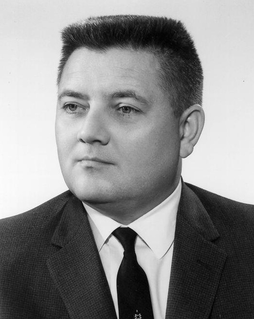
Figure: Ed Jaynes who developed the maximum entropy principle
Maximum Entropy Motivation
Ed Jaynes (Jaynes, 1957), proposed a foundation for statistical mechanics based on information theory. Jaynes recast that the problem of assigning probabilities in statistical mechanics as a problem of inference with incomplete information.
A central problem in statistical mechanics is assigning initial probabilities when our knowledge is incomplete. The canonical example is if we know only the average energy of a system, what probability distribution should we use? Jaynes argued that we should use the distribution that maximises entropy subject to the constraints of our knowledge.
Jaynes illustrated the approach with a simple example. If a die has been tossed many times, with an average result of 4.5 rather than the expected 3.5 for a fair die. What probability assignment \(P_n\) (\(n=1,2,...,6\)) should we make for the next toss?
We need to satisfy two constraints \[\begin{align} \sum_{n=1}^6 P_n &= 1 \\ \sum_{n=1}^6 n P_n &= 4.5 \end{align}\]
Many distributions could satisfy these constraints, but which one makes the fewest unwarranted assumptions? Jaynes argued that we should choose the distribution that is maximally noncommittal with respect to missing information - the one that maximises the entropy, \[\begin{align} S_I = -\sum_{i} p_i \log p_i \end{align}\] This principle leads to the exponential family of distributions, which in statistical mechanics gives us the canonical ensemble and other familiar distributions.
Die Roll Simulation
This simulation illustrates the maximum entropy principle through Jaynes’ dice example (Jaynes, 1957). A fair die has expected outcome 3.5; the Jaynes example asks: if we know only that the average outcome is 4.5, what probability distribution \(P_n\) over the six faces should we assign?
The answer is the maximum-entropy distribution subject to the constraint \(\sum_{n=1}^6 n P_n = 4.5\), which belongs to the exponential family: \[\begin{align} P_n = \frac{e^{\lambda n}}{Z(\lambda)}, \qquad Z(\lambda) = \sum_{n=1}^6 e^{\lambda n} \end{align}\] where \(\lambda > 0\) is chosen so the mean constraint is satisfied. This avoids any unwarranted assumption beyond the available data.
Rolls: 0
Sample mean: —
H(p): —
Outcome weights (auto-normalised to probabilities)
Figure: Interactive die-roll simulation. Click the die or press Roll to sample from the configured distribution. The histogram shows empirical relative frequencies (coloured bars) overlaid on the theoretical probabilities (dashed outlines). Use the sliders to set arbitrary outcome weights, or click a preset to load the uniform distribution (mean 3.5), the Jaynes maximum-entropy distribution (mean 4.5), the simple 50/50 distribution (faces 4 and 5 equally, mean 4.5 with minimal entropy), or a low-biased distribution (mean 2).
The General Maximum-Entropy Formalism
For a more general case, suppose a quantity \(x\) can take values \((x_1, x_2, \ldots, x_n)\) and we know the average values of several functions \(f_k(x)\). The problem is to find the probability assignment \(p_i = p(x_i)\) that satisfies \[\begin{align} \sum_{i=1}^n p_i &= 1 \\ \sum_{i=1}^n p_i f_k(x_i) &= \langle f_k(x) \rangle = F_k \quad k=1,2,\ldots,m \end{align}\] and maximises the entropy \(S_I = -\sum_{i=1}^n p_i \log p_i\).
Using Lagrange multipliers, the solution is the generalised canonical distribution, \[\begin{align} p_i = \frac{\exp(-\lambda_1 f_1(x_i) - \ldots - \lambda_m f_m(x_i))}{Z(\lambda_1,\ldots,\lambda_m)} \end{align}\] where \(Z(\lambda_1,\ldots,\lambda_m)\) is the partition function, \[\begin{align} Z(\lambda_1,\ldots,\lambda_m) = \sum_{i=1}^n \exp(-\lambda_1 f_1(x_i) - \ldots - \lambda_m f_m(x_i)) \end{align}\] The Lagrange multipliers \(\lambda_k\) are determined by the constraints, \[\begin{align} \langle f_k \rangle = -\frac{\partial}{\partial \lambda_k}\log Z(\lambda_1,\ldots,\lambda_m) \quad k=1,2,\ldots,m. \end{align}\] The maximum attainable entropy is \[\begin{align} (S_I)_{max} = \log Z + \sum_{k=1}^m \lambda_k \langle f_k \rangle. \end{align}\]
\[ p_i = \frac{\exp(-\lambda_1 f_1(x_i) - \ldots - \lambda_m f_m(x_i))}{Z(\lambda_1,\ldots,\lambda_m)} \] \[ Z(\ldots) = \sum_{i=1}^n \exp(-\lambda_1 f_1(x_i) - \ldots - \lambda_m f_m(x_i)) \] \[ \langle f_k \rangle = -\frac{\partial}{\partial \lambda_k}\log Z(\lambda_1,\ldots,\lambda_m) \quad k=1,2,\ldots,m. \]
The Classical Observer
Figure: Here the observer is monitoring the movements of the particles. We’ve plotted the velocities alongside the 1 standard deviation contour of their theoretical distribution.
The Classical Observer - Correlated
The Classical Observer - Anti-correlated
Back to self adjudication
The Classical Observer - Inaccessible
Figure: Here the observer is blocked from monitoring anything inside the sytem.
When we don’t know what’s going on inside, we can’t express outcomes in the way we could with an observer. But we can still express entropies. This highlights an interesting characteristic of entropies. If we don’t express the probability directly, but just work with the entropies themselves, it feels like we can assess the bounds of possibility without directly expressing what’s going on.
Joint Entropy
While we don’t see the underlying probability, we can capture a class of different distirbutions by considering the mapping to the system’s joint entropy.
Think of joint entropy as a scoring system: every configuration gets a number measuring its uncertainty. Once you have that, you can line them up from least to most disordered.
The \(I + H = C\) Structure
We have established four axioms, with the fourth axiom stating that the sum of marginal entropies is conserved, \[ \sum_{i=1}^N h_i = C. \] This conservation law is the heart of The Inaccessible Game, but to understand its dynamical implications, we need to rewrite it in a more revealing form.
Multi-Information: Measuring Correlation
The multi-information (or total correlation), introduced by Watanabe (1960), measures how much the variables in a system are correlated. It is defined as, \[ I = \sum_{i=1}^N h_i - H, \] where \(H\) is the joint entropy of the full system: \[ H = -\sum_{\mathbf{x}} p(\mathbf{x}) \log p(\mathbf{x}). \]
The multi-information has a nice interpretation:
- \(I = 0\): The variables are completely independent. The joint entropy equals the sum of marginal entropies.
- \(I > 0\): The variables are correlated. Some information is “shared” between variables, so the joint entropy is less than the sum of marginals.
- \(I\) is maximal: The variables are maximally correlated (in the extreme case, deterministically related).
Multi-information is always non-negative (\(I \geq 0\)) and measures how much knowing one variable tells you about others.
Using the definition of multi-information, we can rewrite our conservation law. From \(I = \sum_{i=1}^N h_i - H\), we have: \[ \sum_{i=1}^N h_i = I + H. \] Therefore, the fourth axiom \(\sum_{i=1}^N h_i = C\) becomes: \[ I + H = C. \]
This is an information action principle. It says that multi-information plus joint entropy is conserved. This equation sits behind the dynamics of the Inaccessible Game.
This equation has the structure of an action principle in classical mechanics. In physics, total energy is conserved and splits into two parts, \[ V + T = E, \] where \(V\) is potential energy and \(T\) is kinetic energy.
The analogy for The Inaccessible Game is.
- Multi-information \(I\) plays the role of potential energy. It represents “stored” correlation structure. High \(I\) means variables are tightly coupled, like a compressed spring.
- Joint entropy \(H\) plays the role of kinetic energy. It represents “dispersed” or “free” information. High \(H\) means the probability distribution is spread out, with maximal uncertainty.
Just as a classical system evolves from high potential energy to high kinetic energy (a ball rolling down a hill), the idea in the Inaccessible Game will be that the information system evolves from high correlation (high \(I\)) to high entropy (high \(H\)).
Entropy Configuration Mapping
Figure: Many configurations (density matrices \(\rho\)) map under von Neumann entropy \(S\) to a single real number. Configurations with the same entropy value are isoentropy; they form an equivalence class. The quotient is a totally ordered chain of entropy levels.
Formally, von Neumann entropy first induces a preorder on configurations \[ \rho \preceq_S \sigma \iff S(\rho) \leq S(\sigma). \] Configurations with equal entropy are mutually comparable, so the preorder is not antisymmetric. Quotienting by the induced equivalence relation \[ \rho \sim_S \sigma \iff S(\rho) = S(\sigma) \] produces a poset of entropy levels, which embeds into \((\mathbb{R}_{\geq 0}, \leq)\). This quotient is the formal entropy ladder.
We can picture the structure as a ladder: each rung corresponds to an entropy level \(S = c\), and multiple configurations sit at the same rung. Moving up the ladder means increasing entropy, more mixed, less structured. Moving down means decreasing entropy, more ordered, more pure.
This picture does not require us to know configuration the system is in at any rung, only the system sits on the ladder. We can think of dynamics in the inaccessible game as being expressed as movement along this ladder.
Figure: The entropy ladder: each rung is an isoentropy class. Multiple configurations sit at the same rung. Dynamics move the system up the ladder (entropy increase) subject to the marginal entropy conservation constraint.
Von Neumann entropy assigns a real value to each configuration, inducing a preorder on the space of density matrices. The quotient by isoentropy equivalence is a totally ordered chain of entropy levels embedded in \((\mathbb{R}_{\geq 0}, \leq)\). The Parzygnat (2022) characterisation establishes that von Neumann entropy is the unique (up to rescaling) continuous, functorial measure of information loss in \(\textsf{NCFinProb}\); this is the information-loss functor, which the entropy-level ordering reflects but is distinct from.
The Exponential Family
An important class of distribution is known as the exponential family. These distributions can be written as \[ p(\mathbf{ y}| \boldsymbol{ \theta}) = \exp(\boldsymbol{ \theta}^\top T- \psi(\boldsymbol{ \theta})) h(\boldsymbol{ \theta}) \] where \(\boldsymbol{ \theta}\) is known as the , \(T(\mathbf{ y})\) is known as the and \(\psi\) is the the log partition function, or the and \(h(\cdot)\) is known as the base measure.
For the moment we’ll ignore the base measure as for several of the distributions we’ll consider it’s constant, so we will consider the form \[ p(\mathbf{ y}| \boldsymbol{ \theta}) = \exp(\boldsymbol{ \theta}^\top T- \psi(\boldsymbol{ \theta})). \] This form yields a particularly simple likelihood function \[ L(\boldsymbol{ \theta}) = \boldsymbol{ \theta}^\top T- \psi(\boldsymbol{ \theta}) \] and since the gradient of the cumulant generating function is the first cumulant of the sufficient statistics, the gradient of the log likelihood also has a simple form. \[ \nabla_\boldsymbol{ \theta}L(\boldsymbol{ \theta}) = T- \left\langle T\right\rangle_{p(\mathbf{ y}|\boldsymbol{ \theta})}. \] where $ denotes the expecttion under the distribution \(p(\cdot)\).
Axiomatically Distinguished
The direction of maximum entropy ascent is the unique steepest-ascent direction in the Fisher (Riemannian) metric. No external structure — no Hamiltonian, no clock, no spatial coordinates — is needed to specify it. Within the inaccessible game framework, this trajectory is axiomatically distinguished: uniquely identifiable under the stated axioms, without introducing external structure (Lawrence, 2025).
The information relaxation principle says the game evolves by maximising joint entropy production subject to the marginal entropy constraint \(\sum_i h_i = C\). In natural parameter space the joint entropy gradient is \[ \nabla H = -G(\boldsymbol{\theta})\boldsymbol{\theta}. \] We enforce the constraint via a Lagrange multiplier \(\nu(\tau)\), giving constrained dynamics \[ \dot{\boldsymbol{\theta}} = -G(\boldsymbol{\theta})\boldsymbol{\theta} + \nu(\tau)\,\mathbf{a}(\boldsymbol{\theta}), \] where \(\mathbf{a}(\boldsymbol{\theta}) = \nabla\!\sum_i h_i\) is the constraint gradient and \(\nu(\tau)\) is determined by requiring \(\mathbf{a}^\top\dot{\boldsymbol{\theta}} = 0\) (the constraint is maintained). Here \(\tau\) is game time, the affine parameter tracking progress along the trajectory.
Long Story Short
Building on these ideas, some interesting conclusions emerge. The marginal engropy constraint leads to GENERIC-like dynamics Öttinger (2005).
When characterising the origin of the game, a shift is forced from Shannon entropy to von Neumann entropy (Neumann, 1932). In retrospect the shift feels natural if we take an algebraic view of quantum probability, where outcomes are no longer primitive. This is consistent with the inaccessible nature of the game.
The game is inspired by the nice connections between inference and thermodynamics explored by E. T. Jaynes, but the dynamics play out through the framework of information geometry (Amari and Nagaoka, 2000) which makes much of the (normally complicated) calculations around Riemanian geometry relatively straightforward.
Energy
Pendulum Animation
import numpy as np# Simple pendulum: trading potential ↔ kinetic energy
# State: angle θ and angular velocity ω
# Energy: E = (1/2)mL²ω² + mgL(1-cos(θ))
# Parameters
g = 9.81 # gravity
L = 1.0 # length
m = 1.0 # mass
# Initial conditions: release from angle, zero velocity
theta0 = np.pi/3 # 60 degrees
omega0 = 0.0
initial_state = np.array([theta0, omega0])
initial_energy = pendulum_energy(theta0, omega0)
# Simulate using Störmer-Verlet method (symplectic integrator, preserves energy)
dt = 0.02
t_max = 5.0
num_steps = int(t_max / dt)
# Arrays to store trajectory
times = np.linspace(0, t_max, num_steps)
trajectory = np.zeros((num_steps, 2))
energies = np.zeros(num_steps)
# Integrate using Störmer-Verlet (symplectic, time-reversible)
# Half-step omega, full-step theta, half-step omega — preserves energy to machine precision
theta, omega = initial_state
for i in range(num_steps):
trajectory[i] = [theta, omega]
energies[i] = pendulum_energy(theta, omega)
omega_half = omega - 0.5 * (g/L) * np.sin(theta) * dt
theta = theta + omega_half * dt
omega = omega_half - 0.5 * (g/L) * np.sin(theta) * dt
# Verify energy conservation
energy_drift = np.abs(energies - initial_energy).max()
print(f"Maximum energy drift: {energy_drift/initial_energy*100:.2f}%")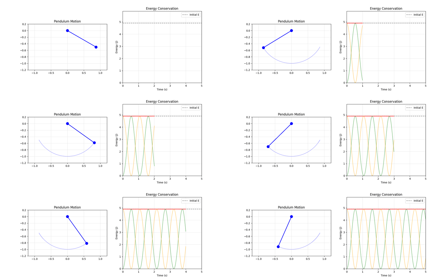
Figure: Pendulum energy conservation: the pendulum (left) trades potential and kinetic energy while total energy (red line, right) remains constant. Green shows kinetic energy, orange shows potential energy.
This pendulum simulation uses.
Energy formula: \(E = \frac{1}{2}mL^2\omega^2 + mgL(1-\cos\theta)\) (kinetic + potential)
Dynamics from energy: The equation \(\frac{\text{d}\omega}{\text{d}t} = -\frac{g}{L}\sin\theta\) comes from energy conservation structure
Trading energy: Watch kinetic (green) and potential (orange) trade off while total (red) stays constant
Geometric structure: The antisymmetric structure we’ll study ensures this conservation automatically
Störmer-Verlet integrator: The simulation uses a symplectic, time-reversible integrator — each step splits the velocity update into two half-steps either side of the position update, preserving the Hamiltonian structure and keeping energy drift at machine precision level.
The animation shows the pendulum swinging with the energy plot demonstrating near-perfect conservation.
One of the nice results of Lawrence (2025) is that in certain thermodynamic limits marginal entropy conservation manifests as energy conservation. So in these (meta-stable) regions one can use Jaynes’ maximum entropy approach to determin the stationary distribution.
Intelligence
Perpetual Motion and Superintelligence
Imagine in 1925 a world where the automobile is already transforming society, but big promises are being made for things to come. The stock market is soaring, the 1918 pandemic is forgotten. And every major automobile manufacturer is investing heavily on the promise they will each be the first to produce a car that needs no fuel. A perpetual motion machine.
Well, of course that didn’t happen. But I sometimes wonder if what we’re seeing today 100 years later is the modern equivalent of that. In 2025 billions are being invested in promises of superintelligence and artificial general intelligence that will transform everything.
We know why perpetual motion is impossible: the second law of thermodynamics tells us that entropy always increases. So we can’t have motion without entropy production. No matter how clever the design, you cannot extract energy from nothing, and you cannot create a closed system that does useful work indefinitely without an external energy source.
How might we make an equivalent statement for the bizarre claims around superintelligence? Some inspiration comes from Maxwell’s demon, an “intelligent” entity which operates against the laws of thermodynamics. The inspiration comes because the demon suggests that for the second law to hold there must be a relationship between the demon’s decisions and thermodynamic entropy.
One of the resolutions comes from Landauer’s principle, the notion that erasure of information requires heat dissipation. This suggests there are fundamental information-theoretic constraints on intelligent systems, just as there are thermodynamic constraints on engines.
I’ve no doubt that AI technologies will transform our world just as much as the automobile has. But I also have no doubt that the promise of superintelligence is just as silly as the promise of perpetual motion. The inaccessible game provides one way of understanding why.
Information-Theoretic Limits
The hope is that this framework might reveal limits on information processing systems, including intelligent systems.
Maxwell’s Demon
Maxwell’s demon is a thought experiment described by James Clerk Maxwell in his book, Theory of Heat (Maxwell, 1871) on page 308.
But if we conceive a being whose faculties are so sharpened that he can follow every molecule in its course, such a being, whose attributes are still as essentially finite as our own, would be able to do what is at present impossible to us. For we have seen that the molecules in a vessel full of air at uniform temperature are moving with velocities by no means uniform, though the mean velocity of any great number of them, arbitrarily selected, is almost exactly uniform. Now let us suppose that such a vessel is divided into two portions, A and B, by a division in which there is a small hole, and that a being, who can see the individual molecules, opens and closes this hole, so as to allow only the swifter molecules to pass from A to B, and the only the slower ones to pass from B to A. He will thus, without expenditure of work, raise the temperature of B and lower that of A, in contradiction to the second law of thermodynamics.
James Clerk Maxwell in Theory of Heat (Maxwell, 1871) page 308
He goes onto say:
This is only one of the instances in which conclusions which we have draw from our experience of bodies consisting of an immense number of molecules may be found not to be applicable to the more delicate observations and experiments which we may suppose made by one who can perceive and handle the individual molecules which we deal with only in large masses
Figure: Maxwell’s demon was designed to highlight the statistical nature of the second law of thermodynamics.
Figure: Maxwell’s Demon. The demon decides balls are either cold (blue) or hot (red) according to their velocity. Balls are allowed to pass the green membrane from right to left only if they are cold, and from left to right only if they are hot. The displayed entropy is the Shannon entropy of the velocity histogram (a coarse-grained proxy, not full thermodynamic entropy).
Maxwell’s demon allows us to connect thermodynamics with information theory (see e.g. Hosoya et al. (2015);Hosoya et al. (2011);Bub (2001);Brillouin (1951);Szilard (1929)). Landauer (1961) described a fundamental connection between information erasure and energy consumption .
Alemi and Fischer (2019)
The perpetual motion analogy provides an accessible way to think about claims of unbounded intelligence.
Information Infrastructures
The information-theoretic constraints that bound individual intelligence extend to collective systems we build. Any institution: organisations, a businesses, government department is an information-processing system embedded subject to the constraints of the information topography. The bottlenecks and channel capacities that constrain what a human can know also constrain what institutions can know, and therefore what they can do.
This was perhaps most famously explored by Stafford Beer whoe developed the Viable System Model Beer (1972), where a cybernetic account of the information channels an organisation must maintain to remain viable. Central to Beer’s analysis is Ashby’s law of requisite variety (Ashby, 1956): the variety of a controller must match the variety of what it seeks to control. Organisations that lack the information bandwidth to track their environment cannot govern themselves effectively.
Recall the embodiment factor introduced earlier: human communication bandwidth is at walking pace while machines operate at light speed. This asymmetry means that the relationship between people and data is now almost always mediated by machine. The information topography of modern organisations is therefore shaped not only by their internal reporting hierarchy, but by the machine infrastructure that now sits between people and the world.
New Flow of Information
Classically the field of statistics focused on mediating the relationship between the machine and the human. Our limited bandwidth of communication means we tend to over-interpret the limited information that we are given, in the extreme we assign motives and desires to inanimate objects (a process known as anthropomorphizing). Much of mathematical statistics was developed to help temper this tendency and understand when we are valid in drawing conclusions from data.
Figure: The trinity of human, data, and computer, and highlights the modern phenomenon. The communication channel between computer and data now has an extremely high bandwidth. The channel between human and computer and the channel between data and human is narrow. New direction of information flow, information is reaching us mediated by the computer. The focus on classical statistics reflected the importance of the direct communication between human and data. The modern challenges of data science emerge when that relationship is being mediated by the machine.
Data science brings new challenges. In particular, there is a very large bandwidth connection between the machine and data. This means that our relationship with data is now commonly being mediated by the machine. Whether this is in the acquisition of new data, which now happens by happenstance rather than with purpose, or the interpretation of that data where we are increasingly relying on machines to summarize what the data contains. This is leading to the emerging field of data science, which must not only deal with the same challenges that mathematical statistics faced in tempering our tendency to over interpret data but must also deal with the possibility that the machine has either inadvertently or maliciously misrepresented the underlying data.
See Lawrence (2024) topography, information p. 34-9, 43-8, 57, 62, 104, 115-16, 127, 140, 192, 196, 199, 291, 334, 354-5. See Lawrence (2024) anthropomorphization (‘anthrox’) p. 30-31, 90-91, 93-4, 100, 132, 148, 153, 163, 216-17, 239, 276, 326, 342.
How Information Flows in Organisations
The information topography of an organisation is how information flows through the organisaiton. At one level this will involve a hierarchy of information propagation: the chart of reporting lines. But alongside this there are other mechanisms to share information.
This dictates the organisations "absorbtive capacity which in turn dictates how it will make decisions. The nature of decisio of decisions depend on how well the information that feeds them can travel.
The three components of the information topography: storage, channel and coupling come together to form the information topography.
Classically information propagates through two principle patterns. Hub-and-spoke networks, and peer-to-peer meshes. The hub-and-spoke becomes a hierarchy as it scales. The different mechanisms have different implications for bandwidth, latency, and resilience.
Figure: In a classical corporate hierarchy, information travels vertically. Strategic decisions flow downward from the CEO through the C-suite (CFO, CIO, COO) to functional departments. Data and reports flow upward. External signals from customers and markets enter at the top. Each layer introduces delay and compression.
The hub-and-spoke model centralises information processing. All communication between departments routes through a central function. This works well for “command and control” but the central node tends to become overloaded. In practive that’s why we obtain a hierarchy so each spoke is itself a hub for the next level.
Figure: In a hub-and-spoke model, all information routes through a central node. This can result in low latency (good command and control) but the central hub can become overloaded.
Peer-to-peer structures allow direct communication between teams without a central intermediary. This maximises bandwidth and reduces latency, but requires more communication interfaces than are managed with hub-and-spoke. Amazon’s API mandate — requiring all teams to expose their capabilities through programmatic interfaces — is an example of deliberately engineering a peer-to-peer information structure within a large organisation. The challenge is coordination: without a hub, norms and protocols must emerge from the network itself. This is where culture becomes important
Figure: In a peer-to-peer network, teams communicate directly with each other through adjacent and cross-cutting channels, without routing through a central authority. This structure is resilient and high-bandwidth, but requires shared protocols and trust. It mirrors how open-source software communities and federated data ecosystems operate.
Conclusions
We began with a tautology — self-governing systems cannot refer to external arbitration — and asked what mathematical structure it forces. The answer, obtained by applying the no-barber principle to information theory, turns out to be surprisingly rich.
No-barber principle. Formalised through the axiomatic frameworks of Baez et al. (2011) and Parzygnat (2022), the requirement of internal adjudicability prohibits outcome spaces, Hamiltonians, clocks, and external observers from appearing as primitives. The game must define everything it uses from within (Lawrence, 2026a).
Information isolation. The no-barber principle suggests the marginal entropy sum \(\sum_i h_i = C\) as a global conservation law.
Axiomatic selection. The game structure requires a pure-state LME origin with positive marginal entropies — a configuration impossible under Shannon entropy (Lawrence, 2026b).
Emergent effective rules. With no Hamiltonian, no clock, and no spatial structure in the axioms, structure emerges. Entropy time provides an internal clock. In Gibbs-locked regions an effective Hamiltonian emerges from the modular generator (Lawrence, 2026c).
Limits on intelligence. By analogy with perpetual motion, information-theoretic constraints bound what any self-contained reasoning system can achieve. A system that cannot refer outside itself cannot access information it has not already processed.
Thanks!
For more information on these subjects and more you might want to check the following resources.
- company: Trent AI
- book: The Atomic Human
- twitter: @lawrennd
- podcast: The Talking Machines
- newspaper: Guardian Profile Page
- blog: http://inverseprobability.com