Abstract

Machine learning solutions, in particular those based on deep learning methods, form an underpinning of the current revolution in “artificial intelligence” that has dominated popular press headlines and is having a significant influence on the wider tech agenda. In this talk I will give an overview of where we are now with machine learning solutions, and what challenges we face both in the near and far future. These include practical application of existing algorithms in the face of the need to explain decision making, mechanisms for improving the quality and availability of data, dealing with large unstructured datasets.

Setup

notutils

This small package is a helper package for various notebook utilities used

The software can be installed using

%pip install notutils

from the command prompt where you can access your python installation.

The code is also available on GitHub: https://github.com/lawrennd/notutils

Once notutils is installed, it can be imported in the usual manner.

import notutils

pods

In Sheffield we created a suite of software tools for ‘Open Data Science’. Open data science is an approach to sharing code, models and data that should make it easier for companies, health professionals and scientists to gain access to data science techniques.

You can also check this blog post on Open Data Science.

The software can be installed using

%pip install pods

from the command prompt where you can access your python installation.

The code is also available on GitHub: https://github.com/lawrennd/ods

Once pods is installed, it can be imported in the usual manner.

import pods

mlai

The mlai software is a suite of helper functions for teaching and demonstrating machine learning algorithms. It was first used in the Machine Learning and Adaptive Intelligence course in Sheffield in 2013.

The software can be installed using

%pip install mlai

from the command prompt where you can access your python installation.

The code is also available on GitHub: https://github.com/lawrennd/mlai

Once mlai is installed, it can be imported in the usual manner.

import mlai

Complexity in Action

As an exercise in understanding complexity, watch the following video. You will see the basketball being bounced around, and the players moving. Your job is to count the passes of those dressed in white and ignore those of the individuals dressed in black.

Figure: Daniel Simon’s famous illusion “monkey business”. Focus on the movement of the ball distracts the viewer from seeing other aspects of the image.

In a classic study Simons and Chabris (1999) ask subjects to count the number of passes of the basketball between players on the team wearing white shirts. Fifty percent of the time, these subjects don’t notice the gorilla moving across the scene.

The phenomenon of inattentional blindness is well known, e.g in their paper Simons and Charbris quote the Hungarian neurologist, Rezsö Bálint,

It is a well-known phenomenon that we do not notice anything happening in our surroundings while being absorbed in the inspection of something; focusing our attention on a certain object may happen to such an extent that we cannot perceive other objects placed in the peripheral parts of our visual field, although the light rays they emit arrive completely at the visual sphere of the cerebral cortex.

Rezsö Bálint 1907 (translated in Husain and Stein 1988, page 91)

When we combine the complexity of the world with our relatively low bandwidth for information, problems can arise. Our focus on what we perceive to be the most important problem can cause us to miss other (potentially vital) contextual information.

This phenomenon is known as selective attention or ‘inattentional blindness’.

Figure: For a longer talk on inattentional bias from Daniel Simons see this video.

Data Selective Attention Bias

We are going to see how inattention biases can play out in data analysis by going through a simple example. The analysis involves body mass index and activity information.

BMI Steps Data

The BMI Steps example is taken from Yanai and Lercher (2020). We are given a data set of body-mass index measurements against step counts. For convenience we have packaged the data so that it can be easily downloaded.

import pods

data = pods.datasets.bmi_steps()
X = data['X'] 
y = data['Y']

It is good practice to give our variables interpretable names so that the analysis may be clearly understood by others. Here the steps count is the first dimension of the covariate, the bmi is the second dimension and the gender is stored in y with 1 for female and 0 for male.

steps = X[:, 0]
bmi = X[:, 1]
gender = y[:, 0]

We can check the mean steps and the mean of the BMI.

print('Steps mean is {mean}.'.format(mean=steps.mean()))

print('BMI mean is {mean}.'.format(mean=bmi.mean()))

BMI Steps Data Analysis

We can also separate out the means from the male and female populations. In python this can be done by setting male and female indices as follows.

male_ind = (gender==0)
female_ind = (gender==1)

And now we can extract the variables for the two populations.

male_steps = steps[male_ind]
male_bmi = bmi[male_ind]

And as before we compute the mean.

print('Male steps mean is {mean}.'.format(mean=male_steps.mean()))

print('Male BMI mean is {mean}.'.format(mean=male_bmi.mean()))

Similarly, we can get the same result for the female portion of the populaton.

female_steps = steps[female_ind]
female_bmi = bmi[female_ind]

print('Female steps mean is {mean}.'.format(mean=female_steps.mean()))

print('Female BMI mean is {mean}.'.format(mean=female_bmi.mean()))

Interesting, the female BMI average is slightly higher than the male BMI average. The number of steps in the male group is higher than that in the female group. Perhaps the steps and the BMI are anti-correlated. The more steps, the lower the BMI.

Python provides a statistics package. We’ll import this in python so that we can try and understand the correlation between the steps and the BMI.

from scipy.stats import pearsonr

corr, _ = pearsonr(steps, bmi)
print("Pearson's overall correlation: {corr}".format(corr=corr))

male_corr, _ = pearsonr(male_steps, male_bmi)
print("Pearson's correlation for males: {corr}".format(corr=male_corr))

female_corr, _ = pearsonr(female_steps, female_bmi)
print("Pearson's correlation for females: {corr}".format(corr=female_corr))

A Hypothesis as a Liability

This analysis is from an article titled “A Hypothesis as a Liability” (Yanai and Lercher, 2020), they start their article with the following quite from Herman Hesse.

“ ‘When someone seeks,’ said Siddhartha, ‘then it easily happens that his eyes see only the thing that he seeks, and he is able to find nothing, to take in nothing. […] Seeking means: having a goal. But finding means: being free, being open, having no goal.’ ”

Hermann Hesse

Their idea is that having a hypothesis can constrain our thinking. However, in answer to their paper Felin et al. (2021) argue that some form of hypothesis is always necessary, suggesting that a hypothesis can be a liability

My view is captured in the introductory chapter to an edited volume on computational systems biology that I worked on with Mark Girolami, Magnus Rattray and Guido Sanguinetti.

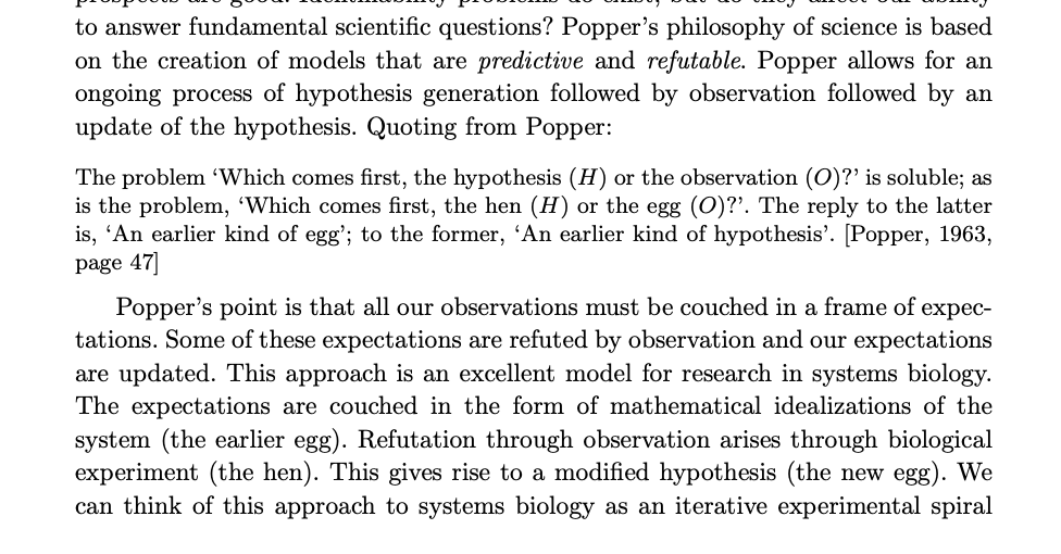
Figure: Quote from Lawrence (2010) highlighting the importance of interaction between data and hypothesis.

Popper nicely captures the interaction between hypothesis and data by relating it to the chicken and the egg. The important thing is that these two co-evolve.

What is Machine Learning?

What is machine learning? At its most basic level machine learning is a combination of

\[\text{data} + \text{model} \stackrel{\text{compute}}{\rightarrow} \text{prediction}\]

where data is our observations. They can be actively or passively acquired (meta-data). The model contains our assumptions, based on previous experience. That experience can be other data, it can come from transfer learning, or it can merely be our beliefs about the regularities of the universe. In humans our models include our inductive biases. The prediction is an action to be taken or a categorization or a quality score. The reason that machine learning has become a mainstay of artificial intelligence is the importance of predictions in artificial intelligence. The data and the model are combined through computation.

In practice we normally perform machine learning using two functions. To combine data with a model we typically make use of:

a prediction function it is used to make the predictions. It includes our beliefs about the regularities of the universe, our assumptions about how the world works, e.g., smoothness, spatial similarities, temporal similarities.

an objective function it defines the ‘cost’ of misprediction. Typically, it includes knowledge about the world’s generating processes (probabilistic objectives) or the costs we pay for mispredictions (empirical risk minimization).

The combination of data and model through the prediction function and the objective function leads to a learning algorithm. The class of prediction functions and objective functions we can make use of is restricted by the algorithms they lead to. If the prediction function or the objective function are too complex, then it can be difficult to find an appropriate learning algorithm. Much of the academic field of machine learning is the quest for new learning algorithms that allow us to bring different types of models and data together.

A useful reference for state of the art in machine learning is the UK Royal Society Report, Machine Learning: Power and Promise of Computers that Learn by Example.

You can also check my post blog post on What is Machine Learning?.

Artificial Intelligence and Data Science

Machine learning technologies have been the driver of two related, but distinct disciplines. The first is data science. Data science is an emerging field that arises from the fact that we now collect so much data by happenstance, rather than by experimental design. Classical statistics is the science of drawing conclusions from data, and to do so statistical experiments are carefully designed. In the modern era we collect so much data that there’s a desire to draw inferences directly from the data.

As well as machine learning, the field of data science draws from statistics, cloud computing, data storage (e.g. streaming data), visualization and data mining.

In contrast, artificial intelligence technologies typically focus on emulating some form of human behaviour, such as understanding an image, or some speech, or translating text from one form to another. The recent advances in artificial intelligence have come from machine learning providing the automation. But in contrast to data science, in artificial intelligence the data is normally collected with the specific task in mind. In this sense it has strong relations to classical statistics.

Classically artificial intelligence worried more about logic and planning and focused less on data driven decision making. Modern machine learning owes more to the field of Cybernetics (Wiener, 1948) than artificial intelligence. Related fields include robotics, speech recognition, language understanding and computer vision.

There are strong overlaps between the fields, the wide availability of data by happenstance makes it easier to collect data for designing AI systems. These relations are coming through wide availability of sensing technologies that are interconnected by cellular networks, WiFi and the internet. This phenomenon is sometimes known as the Internet of Things, but this feels like a dangerous misnomer. We must never forget that we are interconnecting people, not things.

Evolved Relationship with Information

The high bandwidth of computers has resulted in a close relationship between the computer and data. Large amounts of information can flow between the two. The degree to which the computer is mediating our relationship with data means that we should consider it an intermediary.

Originally our low bandwidth relationship with data was affected by two characteristics. Firstly, our tendency to over-interpret driven by our need to extract as much knowledge from our low bandwidth information channel as possible. Secondly, by our improved understanding of the domain of mathematical statistics and how our cognitive biases can mislead us.

With this new set up there is a potential for assimilating far more information via the computer, but the computer can present this to us in various ways. If its motives are not aligned with ours then it can misrepresent the information. This needn’t be nefarious it can be simply because of the computer pursuing a different objective from us. For example, if the computer is aiming to maximize our interaction time that may be a different objective from ours which may be to summarize information in a representative manner in the shortest possible length of time.

For example, for me, it was a common experience to pick up my telephone with the intention of checking when my next appointment was, but to soon find myself distracted by another application on the phone and end up reading something on the internet. By the time I’d finished reading, I would often have forgotten the reason I picked up my phone in the first place.

There are great benefits to be had from the huge amount of information we can unlock from this evolved relationship between us and data. In biology, large scale data sharing has been driven by a revolution in genomic, transcriptomic and epigenomic measurement. The improved inferences that can be drawn through summarizing data by computer have fundamentally changed the nature of biological science, now this phenomenon is also influencing us in our daily lives as data measured by happenstance is increasingly used to characterize us.

Better mediation of this flow requires a better understanding of human-computer interaction. This in turn involves understanding our own intelligence better, what its cognitive biases are and how these might mislead us.

For further thoughts see Guardian article on marketing in the internet era from 2015.

You can also check my blog post on System Zero. This was also written in 2015.

New Flow of Information

Classically the field of statistics focused on mediating the relationship between the machine and the human. Our limited bandwidth of communication means we tend to over-interpret the limited information that we are given, in the extreme we assign motives and desires to inanimate objects (a process known as anthropomorphizing). Much of mathematical statistics was developed to help temper this tendency and understand when we are valid in drawing conclusions from data.

Figure: The trinity of human, data, and computer, and highlights the modern phenomenon. The communication channel between computer and data now has an extremely high bandwidth. The channel between human and computer and the channel between data and human is narrow. New direction of information flow, information is reaching us mediated by the computer. The focus on classical statistics reflected the importance of the direct communication between human and data. The modern challenges of data science emerge when that relationship is being mediated by the machine.

Data science brings new challenges. In particular, there is a very large bandwidth connection between the machine and data. This means that our relationship with data is now commonly being mediated by the machine. Whether this is in the acquisition of new data, which now happens by happenstance rather than with purpose, or the interpretation of that data where we are increasingly relying on machines to summarize what the data contains. This is leading to the emerging field of data science, which must not only deal with the same challenges that mathematical statistics faced in tempering our tendency to over interpret data but must also deal with the possibility that the machine has either inadvertently or maliciously misrepresented the underlying data.

Data Science Africa

Figure: Data Science Africa http://datascienceafrica.org is a ground up initiative for capacity building around data science, machine learning and artificial intelligence on the African continent.

Figure: Data Science Africa meetings held up to October 2021.

Data Science Africa is a bottom up initiative for capacity building in data science, machine learning and artificial intelligence on the African continent.

As of October 2021 there have been five workshops and five schools, located in Nyeri, Kenya (twice); Kampala, Uganda; Arusha, Tanzania; Abuja, Nigeria; Addis Ababa, Ethiopia; Accra, Ghana; Kampala, Uganda and Kimberley, South Africa.

The main notion is end-to-end data science. For example, going from data collection in the farmer’s field to decision making in the Ministry of Agriculture. Or going from malaria disease counts in health centers to medicine distribution.

The philosophy is laid out in (Lawrence, 2015). The key idea is that the modern information infrastructure presents new solutions to old problems. Modes of development change because less capital investment is required to take advantage of this infrastructure. The philosophy is that local capacity building is the right way to leverage these challenges in addressing data science problems in the African context.

Data Science Africa is now a non-govermental organization registered in Kenya. The organising board of the meeting is entirely made up of scientists and academics based on the African continent.

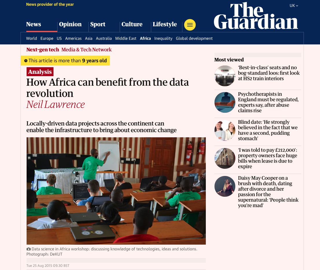
Figure: The lack of existing physical infrastructure on the African continent makes it a particularly interesting environment for deploying solutions based on the information infrastructure. The idea is explored more in this Guardian op-ed on Guardian article on How African can benefit from the data revolution.

Guardian article on Data Science Africa

Example: Prediction of Malaria Incidence in Uganda

As an example of using Gaussian process models within the full pipeline from data to decsion, we’ll consider the prediction of Malaria incidence in Uganda. For the purposes of this study malaria reports come in two forms, HMIS reports from health centres and Sentinel data, which is curated by the WHO. There are limited sentinel sites and many HMIS sites.

The work is from Ricardo Andrade Pacheco’s PhD thesis, completed in collaboration with John Quinn and Martin Mubangizi (Andrade-Pacheco et al., 2014; Mubangizi et al., 2014). John and Martin were initally from the AI-DEV group from the University of Makerere in Kampala and more latterly they were based at UN Global Pulse in Kampala. You can see the work summarized on the UN Global Pulse disease outbreaks project site here.

• See UN Global Pulse Disease Outbreaks Site

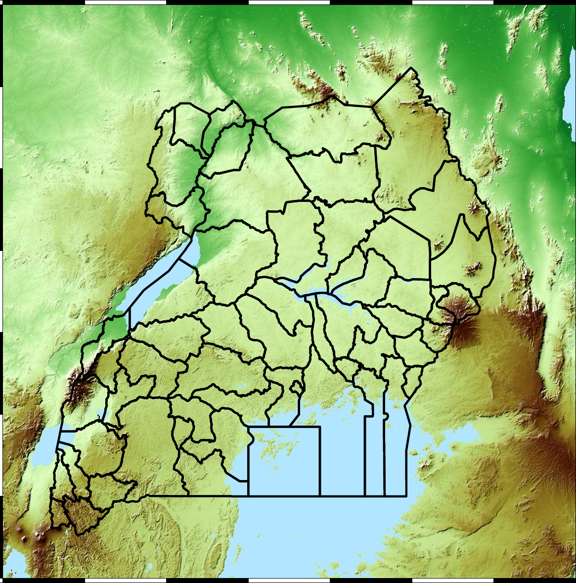
Malaria data is spatial data. Uganda is split into districts, and health reports can be found for each district. This suggests that models such as conditional random fields could be used for spatial modelling, but there are two complexities with this. First of all, occasionally districts split into two. Secondly, sentinel sites are a specific location within a district, such as Nagongera which is a sentinel site based in the Tororo district.

Figure: Ugandan districts. Data SRTM/NASA from https://dds.cr.usgs.gov/srtm/version2_1.

The common standard for collecting health data on the African continent is from the Health management information systems (HMIS). However, this data suffers from missing values (Gething et al., 2006) and diagnosis of diseases like typhoid and malaria may be confounded.

Figure: The Tororo district, where the sentinel site, Nagongera, is located.

World Health Organization Sentinel Surveillance systems are set up “when high-quality data are needed about a particular disease that cannot be obtained through a passive system”. Several sentinel sites give accurate assessment of malaria disease levels in Uganda, including a site in Nagongera.

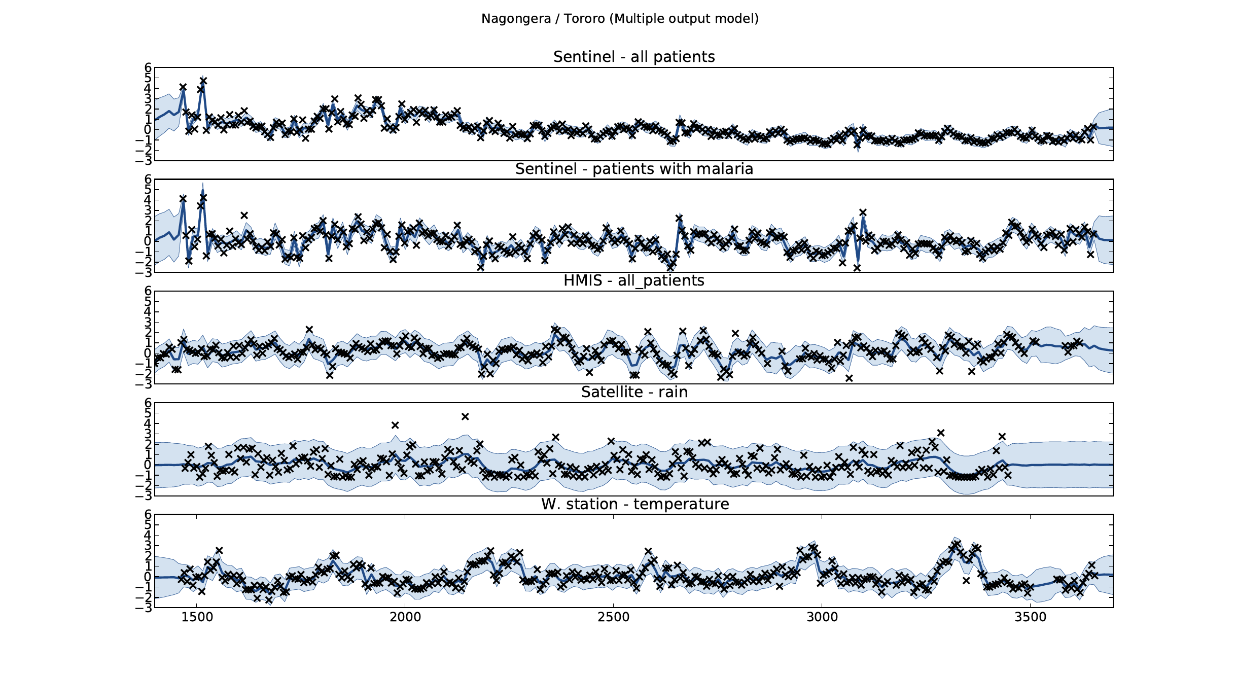
Figure: Sentinel and HMIS data along with rainfall and temperature for the Nagongera sentinel station in the Tororo district.

In collaboration with the AI Research Group at Makerere we chose to investigate whether Gaussian process models could be used to assimilate information from these two different sources of disease informaton. Further, we were interested in whether local information on rainfall and temperature could be used to improve malaria estimates.

The aim of the project was to use WHO Sentinel sites, alongside rainfall and temperature, to improve predictions from HMIS data of levels of malaria.

Figure: The Mubende District.

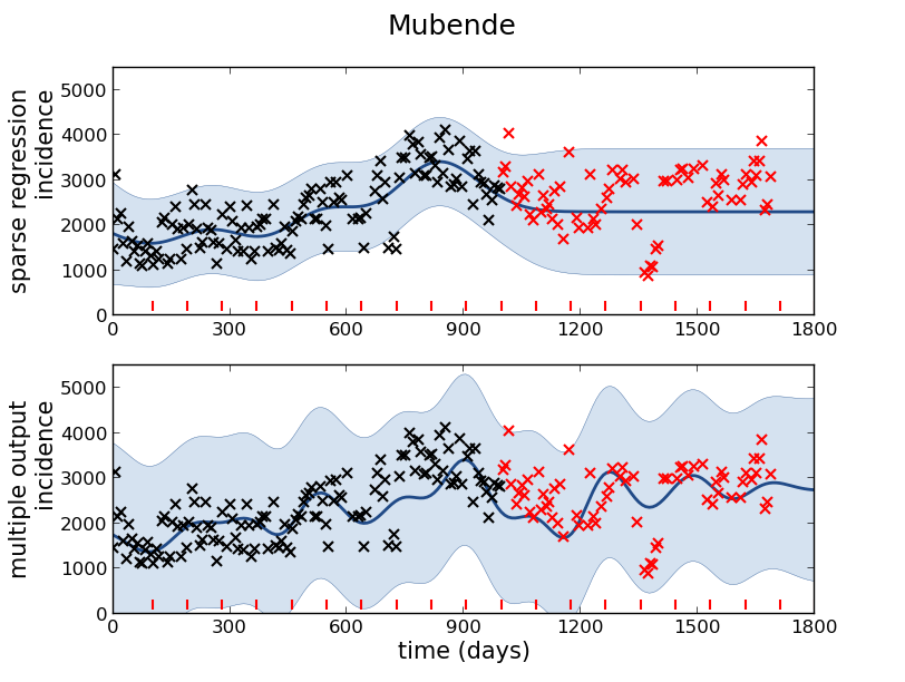
Figure: Prediction of malaria incidence in Mubende.

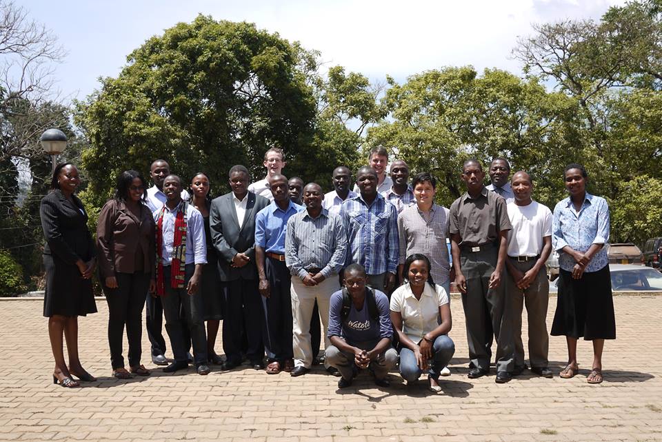
Figure: The project arose out of the Gaussian process summer school held at Makerere in Kampala in 2013. The school led, in turn, to the Data Science Africa initiative.

Early Warning Systems

Figure: The Kabarole district in Uganda.

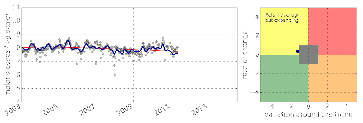
Figure: Estimate of the current disease situation in the Kabarole district over time. Estimate is constructed with a Gaussian process with an additive covariance funciton.

Health monitoring system for the Kabarole district. Here we have fitted the reports with a Gaussian process with an additive covariance function. It has two components, one is a long time scale component (in red above) the other is a short time scale component (in blue).

Monitoring proceeds by considering two aspects of the curve. Is the blue line (the short term report signal) above the red (which represents the long term trend? If so we have higher than expected reports. If this is the case and the gradient is still positive (i.e. reports are going up) we encode this with a red color. If it is the case and the gradient of the blue line is negative (i.e. reports are going down) we encode this with an amber color. Conversely, if the blue line is below the red and decreasing, we color green. On the other hand if it is below red but increasing, we color yellow.

This gives us an early warning system for disease. Red is a bad situation getting worse, amber is bad, but improving. Green is good and getting better and yellow good but degrading.

Finally, there is a gray region which represents when the scale of the effect is small.

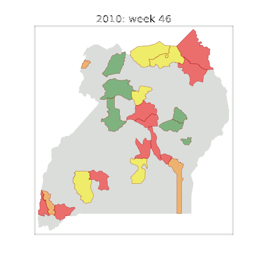
Figure: The map of Ugandan districts with an overview of the Malaria situation in each district.

These colors can now be observed directly on a spatial map of the districts to give an immediate impression of the current status of the disease across the country.

Thanks!

For more information on these subjects and more you might want to check the following resources.

• twitter: @lawrennd
• podcast: The Talking Machines
• newspaper: Guardian Profile Page
• blog: http://inverseprobability.com

References